
My goal here was to look under the hood of principal component analysis (PCA) and get a better sense of how it functions, more specifically in the field of image compression. Using an implementation from scikit-learn, PCA and support vector machines (SVM) were utilized to reduce the dimensionality of and classify over 13,000 color images of famous figures’ faces and look at a rudimentary facial recognition process. PCA utilizes the eigenvectors of the covariance matrix to redescribe data points in the direction of highest variance. A metric developed using a weighted average of precision and recall yielded a score of 77% when 50 principal components were used for the study and out of 36 faces given to the model to recognize, 29 were predicted correctly. Improvements of the study could be developed using a cross-validation of the number of principal components.
Data
Our data are images set to 250 x 250 pixels containing faces of famous figures. There are 13,233 images in the whole set with 5749 different people and 1680 of them contain more than 1 image in their set of images. This is an important fact because the program learns from the images and the highest variance will be described in the direction of people with the most images. The dataset contains 5 errors, which are, Fold 1: Janica_Kostelic_0001, Janica_Kostelic_0002 Fold 1: Nora_Bendijo_0001, Nora_Bendijo_0002 Fold 5: Jim_OBrien_0001, Jim_OBrien_0002 Fold 5: Jim_OBrien_0001, Jim_OBrien_0003 Fold 5: Elisabeth_Schumacher_0001, Elisabeth_Schumacher_0002.
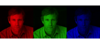
If we are representing our images as a vector of values. Each value corresponds to a pixel’s intensity on a scale measured from 0 to 255 inclusive, and a square $N$ by $N$ image can be expressed as an $N^2$-dimensional vector, \(X = (x_1 x_2 x_3 ... x_{N^2})\) where the rows of pixels are just placed concurrently to form a one dimensional image. We are using color images so we need matrices for each of the three color channels in the RGB color space (red, green, blue). To describe how the data is processed, and a slight introduction into visualizing principal component analysis (PCA), we can take a brief view into one of the images, Aaron Eckhart.
Example


## Importance of components:
##                           PC1     PC2     PC3
## Standard deviation     1.6929 0.36422 0.03701
## Proportion of Variance 0.9553 0.04422 0.00046
## Cumulative Proportion  0.9553 0.99954 1.00000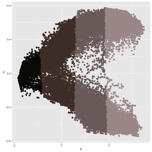
Here we see our segmented image described graphically as a function of its first two principal components $u$ and $v$, respectively. So now that we have seen what PCA can do with one of our training images, lets take a look at how PCA actually works.
What is PCA?
PCA is a technique that identifies patterns in data, and then expresses the data in such a way that highlights these patterns. Some may recognize that identifying patterns in high-dimensionality is a difficult task. Why is this difficult? We cannot display our data visually and the higher we go in dimensions, the more uniformly distant each data point is from every other data point. PCA can be used to reduce this dimensionlity.
Math of PCA
So mathematically, what does PCA want? PCA wants to know if there is another basis that is a linear combination of the original basis, which reexpresses our data. PCA does carry some assumptions with it. One of which is linearity. Linearity makes the problem simpler by reducing the number of possible bases allowed. Linearity also is a benefit that allows us to assume continuity in a data set. If we let X and Y be $m$×$n$ matrices related by a linear transformation $P$, where X is the original data set and Y is a new representation of the data, then,
\(PX=Y\),
$p_i$ are the rows of $P$
$x_i$ are the columns of $X$
$y_i$ are the columns of $Y$
represents a change of basis. The rows of P, ${p1, . . . , pm}$, are a set of new basis vectors for expressing the columns of $X$ and each coefficient of $y_i$ is a dot product of $x_i$ with the corresponding row in $P$. So the jth coefficient of $y_i$ is a projection on to the jth row of $P$, or $y_i$ is a projection on to the basis of ${p1, . . . , pm}$. So our conclusion here is that the rows of $P$ are a new set of basis vectors for the columns of $X$. So we must now ask ourselves, how do we find the correct change of basis? The row vectors ${p1, . . . , pm}$ become the principal components.
The first step in applying PCA on a dataset is to subtract the mean from each of the data dimensions. Where the mean is the average across each dimension. Essentially what this does is produces a data set whose mean is zero.
Our next step is calculating the covariance matrix. PCA is all about variance. Let’s take a look at the idea of variance for a moment.
The variance of A and B are individually defined as follows.
\[\sigma_A^2 = \langle a_i a_i \rangle_i , \sigma_B^2 = \langle b_i b_i \rangle_i\]where the expectation is the average over $n$ variables.
Covariance is much like variance, except instead of seeing how much one variable varies it determines how much two variables ‘co-vary’.
covariance of A and B \(\equiv \sigma_{AB}^2 = \langle a_i b_i \rangle_i\)
But we don’t just want A and B. We want to be able to have a big matrix of $m$ row vectors. So say we make the sets of A and B into row vectors, $a = [a_1, a_2, . . . a_n], b = [b_1, b_2, . . . b_n]$. Now,
\[\sigma_{ab}^2 \equiv \frac{1}{n-1}ab^T\]with the first term for normalization.
Now we can accomplish the expansion of our method from just two vectors to $m$ vectors. We can rename the row vectors $x_1 \equiv a, x_2 \equiv b$ and consider additional indexed row vectors $x3, . . . , xm$. Recall we want a covariance matrix, so we can define a new $m$×$n$ matrix X where each row of X corresponds to all measurements of a particular type ($x_i$). Each column of X corresponds to a set of measurements from one particular trial. And we can call this new matrix the covariance matrix $S_X$,
\[S_X \equiv \frac{1}{n-1}XX^T\]the ijth element of the variance is the dot product between the vector of the ith measurement type with the vector of the jth measurement type.
Now our new matrix $S_X$ gives us correlation information for all possible pairs of values where zero covariance corresponds to entirely uncorrelated data. In a way, we can view our really high-dimensions data set as being extremely redundant, as in, we really don’t need all of those dimensions to describe most of the relationships within the data. So to reduce this redundancy, we can imagine changing the covariance matrix around until each variable co-varies as little as possible with the other variables. So with this new covariance matrix $S_Y$, what features would we want to optimize the most? If we are trying to make the covariances between different values to be zero, this would make all off-diagonal terms in $S_Y$ zero. Or in other words, this ‘diagnolizes’ $S_Y$. To do this, PCA assumes $P$ is an orthonormal matrix, i.e. PCA assumes that all basis vectors ${p1, . . . , pm}$ are orthonormal ($p_i p_j = \delta_{ij}$). The other assumption that PCA makes is that the most important directions are the ones with the largest variances.
So this choice of assuming the directions iwth the highest variances are the most important ones is another way of saying they are the ‘principal’ components. PCA finds the normalized direction that the variance in $X$ is maximized and this is $p_1$ or the first principal component. Then when it goes to select its next direction it must pick a direction that is perpendicular to all previous directions because of the orthonormality condition. We then have to specify how many times it does this. It could select directions up to $m$ times in $m$-dimensions.
So we have calculated the covariance matrix, which will be $p$x$p$, and since this is a square matrix we can calculate the eigenvectors and eigenvalues (note: these are unit eigenvectors). So this extraction of the eigenvectors of the covariance matrix is what gives us the lines that characterize the data. Then we transform the data to be expressed in terms of those directions. We can see that the eigenvector with the greatest eigenvalue is the first principal component. So naturally we want to order the eigenvectors by eigenvalue. Now we have all of the directions in order from most important to least important. So this is the important aspect to dimensionality reduction. We can leave out as many of these components as we want, and that will be the new dimensionality of our data set. Using matrices, this is equivalent to choosing the eigenvectors that we want to keep as our principal components and placing them in a matrix of vecotrs, then take the transpose of thise and multiply it by the original data set, transposed. This will give us the original data in terms of the vectors we chose. Now our data is expressed in terms of the similarities and differences of the data themselves.
Solving PCA. Let’s assume some data set is an $m$×$n$ matrix X, where $m$ is the number of measurement types and $n$ is the number of data trials. The goal is to find some orthonormal matrix P where $Y=PX$ such that $S_Y \equiv \frac{1}{n-1}YY^T$ is diagonalized. The rows of P are the principal components of X. We begin by rewriting $S_Y$ in terms of P.
\[S_Y = \frac{1}{n-1}YY^T\] \[= \frac{1}{n-1}(PX)(PX)^T\] \[= \frac{1}{n-1}P(XX^T)P^T\] \[S_Y = \frac{1}{n-1}PAP^T\]$A \equiv XX^T$ where A is symmetric (A symmetric matrix is diagonalized by an orthogonal matrix of its eigenvectors)
\[A = EDE^T\]where $D$ is a diagonal matrix and $E$ is a matrix of eigenvectors of $A$ arranged as columns. We select the matrix P to be a matrix where each row $p_i$ is an eigenvector of $XX^T$. By this selection, $P \equiv E^T$. Substituting, $A=P^TDP$ and then ($P^{-1} = P^T$),
\[S_Y = \frac{1}{n-1}PAP^T\] \[= \frac{1}{n-1}P(P^TDP)P^T\] \[= \frac{1}{n-1}(PP^T)D(PP^T)\] \[= \frac{1}{n-1}(PP^{-1})D(PP^{-1})\] \[S_Y = \frac{1}{n-1}D\]The choice of P diagonalizes $S_Y$.
PCA for Image Compression
So when we use PCA for image compression, what we are doing is reducing the image to only the most important directions of variance, however we sometimes need to be able to reconstruct the image afterwards. For this we must take all $m$ components when performing PCA, since if we didn’t take all of the components we would have lost some information about the image. To get the original data back we just need to multiply the final data by the inverse of the matrix of vectors we created, then we have to add on the mean of the original data that we subtracted in the beginning.
In our experiment we have varying numbers of images for each famous figure, where each image is 250 pixels wide by 250 pixels high. For each image we create an image vector as described above, and then we put all of the images together in one matrix with each row as an image’s vector. So now assume we have a matrix for each famous person in our set, and then we have performed PCA so we have or original data in terms of the eigenvectors of the covariance matrix. Now we want to use this new information to perform facial recognition on an image or multiple images that the program has never seen before. The program checks for the difference between the new image and the original images, along the new axes determined by PCA eigenvectors directions. This allows the program to check for the most similarities and differences at once since these are the directions of highest variance.
Results
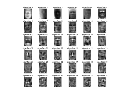
This example of PCA is exciting because we actually have a visual representation of what happened to our photos. The eigenfaces figure below shows how PCA applied to all ~13,000 images has created a kind of compilation photo for all of the famous people, where the most prevalent figures have the most impact on the first eigenface. The first eigenface contains 21.7% of the variance explained and the second component contains 13.6% of the variance explained.
Eigenfaces
Below, we can see a list of 19 figures used in the prediction process and the model’s precision and recall. There is also another metric, f1-score, which can be interpreted as a weighted average of the precision and recall, where an f1 score reaches its best value at 1 and worst score at 0. The relative contribution of precision and recall to the f1 score are equal. The formula for the f1 score is: $f1 = 2 \cdot (\text{precision} \cdot \text{recall}) / (\text{precision} + \text{recall})$. Support is the number of images used for each figure during the classification. The greatest f1-score came with Gloria Macapagal Arroyo and the most comical prediction was the model thought Former Governor of Missouri John Ashcroft was Former Governor of California Arnold Schwarzenegger.
                         precision    recall  f1-score   support

         Ariel Sharon       0.73      0.76      0.74        21
       Schwarzenegger       0.33      0.67      0.44         6
         Colin Powell       0.76      0.75      0.75        67
      Donald Rumsfeld       0.68      0.92      0.78        25
        George W Bush       0.83      0.85      0.84       138
    Gerhard Schroeder       0.86      0.74      0.79        34
            GM Arroyo       0.91      1.00      0.95        10
          Hugo Chavez       0.62      0.76      0.68        17
       Jacques Chirac       0.50      0.50      0.50        10
        Jean Chretien       0.89      0.57      0.70        14
    Jennifer Capriati       0.80      0.57      0.67        14
        John Ashcroft       0.70      0.64      0.67        11
    Junichiro Koizumi       0.92      0.71      0.80        17
           Laura Bush       1.00      0.71      0.83        14
       Lleyton Hewitt       0.44      0.67      0.53         6
         LIL da Silva       0.70      0.64      0.67        11
      Serena Williams       1.00      0.38      0.56        13
           Tony Blair       0.59      0.74      0.66        27
       Vladimir Putin       0.55      0.50      0.52        12
150comp's:avg / total       0.77      0.75      0.75       467
 50comp's:avg / total       0.78      0.77      0.77       467
250comp's:avg / total       0.76      0.75      0.75       467
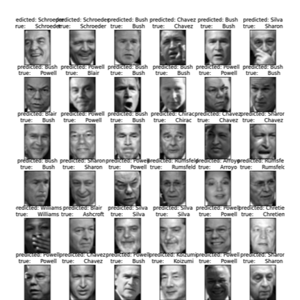
What we can see from the results above is that when the number of principal components was reduced from 150 to 50, there was actually an improved f1-score. A possible reason for this is overfitting. When you allow too much training in the model we can see that the model will only be able to predict those images that it trained on (which is not helpful at all). When we reduce the number of components to 50 we actually see an improved prediction, precision, and recall. When 150 components were used, the model predicted 28 of the 36 images correctly and when 50 components were used the model predicted 29 of the 36 images correctly (see below for 150 components results). With 250 components the model makes 10 errors, only predicting 26 of the 36 correctly.
Predictions
Reference
http://setosa.io/ev/principal-component-analysis/
https://www.cs.princeton.edu/picasso/mats/PCA-Tutorial-Intuition_jp.pdf
Scikit-learn: Machine Learning in Python, Pedregosa et al., JMLR 12, pp. 2825-2830, 2011. http://scikit-learn.org/stable/auto_examples/applications/face_recognition.html