
The primary goals of this report are to obtain the best linear model possible to predict area burnt during forest fires in Montesinho natural park in the Tr´as-os-Montes northeast region of Portugal and to understand the underlying relationships between our predictors and area burnt (i.e. how does area burnt change based on a 1 unit increase in some other variable). Our predicors range from meteorological to temporal to geographical. Predicting forest fires has long been considered a challenging task from statisticians, as so many factors go into its spread and capacity. However, we will always be desperate for simple predictors since the resources to put new technology in various parts of the world are sparce. In this paper, I employed subset selection techniques along with cross validation to build the best linear model possible. I conclude that the best model contains ten predictors. This model results in an RMSE value of about 1.39 and an MAE of 1.155, which is our preferred method of error diagnostics for this dataset (see explanation in section Subset Selection Cross Validates).
library(dplyr)
library(ggplot2)
library(leaps)
library(knitr)
library(caret)
library(corrplot)
set.seed(123)
Variable Descriptions:
- X - x-axis spatial coordinate within the Montesinho park map: 1 to 9
- Y - y-axis spatial coordinate within the Montesinho park map: 2 to 9
- month - month of the year: “jan” to “dec”
- day - day of the week: “mon” to “sun”
- FFMC - Fine Fuel Moisture Code (FFMC) index from the Fire Weather Index (FWI) system: 18.7 to 96.20
- DMC - Duff Moisture Code (DMC) index from the FWI system: 1.1 to 291.3
- DC - Drought Code (DC) index from the FWI system: 7.9 to 860.6
- ISI - Initial Spread Index (ISI) from the FWI system: 0.0 to 56.10
- temp - temperature in Celsius degrees: 2.2 to 33.30
- RH - relative humidity in %: 15.0 to 100
- wind - wind speed in km/h: 0.40 to 9.40
- rain2 - outside rain in mm/m2 : 0.0 to 6.4
- area - the burned area of the forest (in ha): 0.00 to 1090.84
ff <- read.csv("forestfires.csv")
ff2 <- ff %>% mutate(rain2 = as.factor(rain > 0), logarea = log(area + 1)) %>% select(-c(rain, area))
dim(ff2)
## [1] 517 13str(ff2)## 'data.frame': 517 obs. of 13 variables:
## $ X : int 7 7 7 8 8 8 8 8 8 7 ...
## $ Y : int 5 4 4 6 6 6 6 6 6 5 ...
## $ month : Factor w/ 12 levels "apr","aug","dec",..: 8 11 11 8 8 2 2 2 12 12 ...
## $ day : Factor w/ 7 levels "fri","mon","sat",..: 1 6 3 1 4 4 2 2 6 3 ...
## $ FFMC : num 86.2 90.6 90.6 91.7 89.3 92.3 92.3 91.5 91 92.5 ...
## $ DMC : num 26.2 35.4 43.7 33.3 51.3 ...
## $ DC : num 94.3 669.1 686.9 77.5 102.2 ...
## $ ISI : num 5.1 6.7 6.7 9 9.6 14.7 8.5 10.7 7 7.1 ...
## $ temp : num 8.2 18 14.6 8.3 11.4 22.2 24.1 8 13.1 22.8 ...
## $ RH : int 51 33 33 97 99 29 27 86 63 40 ...
## $ wind : num 6.7 0.9 1.3 4 1.8 5.4 3.1 2.2 5.4 4 ...
## $ rain2 : Factor w/ 2 levels "FALSE","TRUE": 1 1 1 2 1 1 1 1 1 1 ...
## $ logarea: num 0 0 0 0 0 0 0 0 0 0 ...We can see that our initial dataset contains 13 variables with 517 observations.
We also have some factor variables alongside of integer and numeric variables.
We will be using the log transform of area burnt (in hectares) due to its strong right skew, and we will be using rain as a factor variable (i.e. whether or not it is raining at the time of the fire).
pairs(ff2[,c(3,4,12,13)])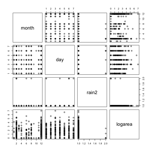
corpears.mat <- cor(ff2[,c(1,2,5,6,7,8,9,10,11,13)])
corspear.mat <- cor(ff2[,c(1,2,5,6,7,8,9,10,11,13)], method = "spearman")par(mfrow=c(1,2))
corrplot(corpears.mat, order = 'hclust')
corrplot(corspear.mat, order = 'hclust')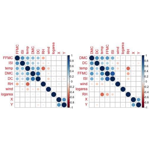
The pairs plot is for the factor variables and the correlation plot is for the numeric variables. The pairs plot indicated no correlation within the factor variables. For the numeric variables, it’s always good practice to run both Pearson and Spearman because Pearson deals with linear relationships so it may falter in some non-linear scenarios where Spearman will not. So, if we have a situation where the Spearman is greater than the Pearson, this indicates that there is something non-linear going on and we may need a log transform on a variable or more. From the plots it seems that many of the meteorological indices are somewhat correlated.
Based on my intimate knowledge of the dataset and the predicor variables, I do not feel that it is necessary to include interaction terms for this model.
trainIndex <- createDataPartition(ff2$logarea, p=0.9, list = FALSE)
ff2Train <- ff2[trainIndex,]
ff2Test <- ff2[-trainIndex,]
full.model <- lm(logarea ~ ., data = ff2Train)
summary(full.model)$coef## Estimate Std. Error t value Pr(>|t|)
## (Intercept) -1.990699673 1.758678719 -1.13192913 0.258280735
## X 0.047602316 0.034087347 1.39648051 0.163273885
## Y -0.013400449 0.063750072 -0.21020289 0.833606629
## monthaug 0.256022739 0.876126141 0.29222132 0.770255148
## monthdec 2.544425811 0.938927128 2.70992895 0.006992696
## monthfeb 0.374492686 0.609073788 0.61485602 0.538967644
## monthjan 0.082615617 1.256826937 0.06573349 0.947619867
## monthjul 0.014948095 0.757433399 0.01973519 0.984263562
## monthjun -0.210677600 0.700882955 -0.30058885 0.763870013
## monthmar -0.157124455 0.546126178 -0.28770724 0.773706308
## monthmay 0.746945499 1.132253722 0.65969798 0.509792806
## monthnov -0.879837033 1.513250648 -0.58142188 0.561253884
## monthoct 0.770504879 1.039469099 0.74124847 0.458938222
## monthsep 0.909968775 0.977237349 0.93116455 0.352279073
## daymon 0.220184849 0.248289127 0.88680826 0.375666586
## daysat 0.314888837 0.235006770 1.33991390 0.180964902
## daysun 0.222382991 0.223447868 0.99523434 0.320169301
## daythu 0.094087455 0.252976471 0.37192176 0.710130149
## daytue 0.411475188 0.245248501 1.67778880 0.094098455
## daywed 0.191922597 0.263779937 0.72758603 0.467254008
## FFMC 0.014370026 0.017165485 0.83714653 0.402964663
## DMC 0.004051423 0.001958798 2.06832064 0.039193599
## DC -0.001743149 0.001329022 -1.31160264 0.190338202
## ISI -0.026935046 0.019017776 -1.41630896 0.157392603
## temp 0.061885533 0.024256997 2.55124456 0.011071236
## RH 0.006017405 0.007127721 0.84422564 0.399002094
## wind 0.079535843 0.041660192 1.90915688 0.056892046
## rain2TRUE -0.971484397 0.622693231 -1.56013322 0.119447339Fitting our full model, we can see the p-values indicate that monthdec, DMC, and temp are significant at the 0.05 level. The $R^2_a$ indicates that about 3% of the variance in the response is explained by a linear relationship with the predictors. This $R^2_a$ is very low, so we shouldn’t expect much from our predictions, but we have a p-value of 0.049 for the current full model so we may be able to see some relationships between the predictors and the response. The residual plot indicated the model needs tweaking.
Nested F-Tests, Forward Selection
add1(lm(logarea ~ temp, data = ff2Train), logarea ~
       X + Y + month + day + FFMC + DMC + DC + ISI +
       temp + RH + wind + rain2, test = "F")
## Single term additions
##
## Model:
## logarea ~ temp
## Df Sum of Sq RSS AIC F value Pr(>F)
## <none> 936.77 328.78
## X 1 3.482 933.29 329.04 1.7347 0.18846
## Y 1 1.228 935.54 330.16 0.6105 0.43501
## month 11 35.773 901.00 332.56 1.6423 0.08417 .
## day 6 4.495 932.28 338.53 0.3696 0.89820
## FFMC 1 0.539 936.23 330.51 0.2676 0.60517
## DMC 1 3.268 933.50 329.14 1.6280 0.20262
## DC 1 1.977 934.79 329.79 0.9834 0.32188
## ISI 1 3.352 933.42 329.10 1.6696 0.19695
## RH 1 0.001 936.77 330.78 0.0005 0.98276
## wind 1 5.013 931.76 328.27 2.5018 0.11440
## rain2 1 1.995 934.78 329.78 0.9922 0.31973
## ---
## Signif. codes: 0 '***' 0.001 '**' 0.01 '*' 0.05 '.' 0.1 ' ' 1Nested F-tests with forward selection indicates the one-variable model with logarea ~ temp.
Nested F-Tests, Backward Selection
Nested F-tests with backward selection also indicates the one-variable model with logarea ~ temp. The order of removal was: Y, day, FFMC, RH, rain2, ISI, DC, X, wind, DMC, month, leaving us with,
drop1(lm(logarea ~ temp, data = ff2Train), test = "F")## Single term deletions
##
## Model:
## logarea ~ temp
## Df Sum of Sq RSS AIC F value Pr(>F)
## <none> 936.77 328.78
## temp 1 9.0918 945.86 331.30 4.5228 0.03397 *
## ---
## Signif. codes: 0 '***' 0.001 '**' 0.01 '*' 0.05 '.' 0.1 ' ' 1Subset Selection Cross Validated (90% Train, 10% Test)
#best subset
ff2.bestsub <- regsubsets(logarea ~ ., data=ff2Train, nvmax = 20)
ff2.bestsub.summary <- summary(ff2.bestsub)
best.cp <- which.min(ff2.bestsub.summary$cp)
cat("The best number of variables to minimize Cp is", best.cp)
best.ar2 <- which.max(ff2.bestsub.summary$adjr2)
cat("The best number of variables to maximize adjusted R^2 is", best.ar2)
best.bic <- which.min(ff2.bestsub.summary$bic)
cat("The best number of variables to minimize BIC is", best.bic)par(mfrow=c(2,2))
plot(ff2.bestsub, scale = 'r2')
plot(ff2.bestsub, scale = 'adjr2')
plot(ff2.bestsub, scale = 'Cp')
plot(ff2.bestsub, scale = 'bic')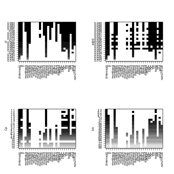
ff2.bestsub.total = regsubsets(logarea ~ ., data = ff2, nvmax = 20)
cat("The coefficients to minimize Cp are\n",
    names(coef(ff2.bestsub.total, 5)))
## The coefficients to minimize Cp are
## (Intercept) X monthdec monthsep temp windcat("The coefficients to maximize adjusted R^2 are\n",
names(coef(ff2.bestsub.total, 12)))## The coefficients to maximize adjusted R^2 are
## (Intercept) X monthdec monthjun monthmar monthoct monthsep daytue DMC DC temp wind rain2TRUEcat("The coefficients to minimize BIC are\n",
names(coef(ff2.bestsub.total, 2)))## The coefficients to minimize BIC are
## (Intercept) monthdec tempOptimizing for $C_p$ (5 vars), $R^2_a$ (12), and $BIC$ (2) are all giving us different models. Let’s continue.
test.mat = model.matrix(logarea ~ ., data = ff2Test)
val.errors = rep(NA, 20)
for(i in 1:20){
  coefi = coef(ff2.bestsub, id=i)
  pred = test.mat[,names(coefi)]%*%coefi
  val.errors[i] = mean((ff2Test$logarea-pred)^2)
}
val.errors.mae = rep(NA, 20)
for(i in 1:20){
coefi = coef(ff2.bestsub, id=i)
pred.mae = test.mat[,names(coefi)]%*%coefi
val.errors.mae[i] = mean(abs(ff2Test$logarea-pred.mae))
}par(mfrow=c(1,2))
plot(val.errors, type = "b")
plot(val.errors.mae, type = "b")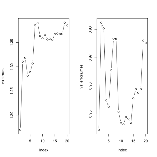
coef(ff2.bestsub, 1)## (Intercept) monthdec
## 1.109950 1.625311coef(ff2.bestsub, 11)## (Intercept) X monthdec monthfeb monthsep
## -0.3372121759 0.0458164419 2.1928116636 0.4398217503 0.4614473719
## daytue DMC DC ISI temp
## 0.2189178855 0.0033051963 -0.0006118161 -0.0226146870 0.0478136280
## wind rain2TRUE
## 0.0729525694 -0.8450540019Here we create matrices from our data to compute the test Mean Square Error (MSE) and Mean Absolute Error (MAE) for each optimal 1-,2-,3-,… variable models. Now I will argue that the MAE is better for our dataset than the MSE. Our response variable, area burnt, contains many 0-values and then occasional large values. The issue with using MSE for data such as this is that we are relying too heavily on the error terms for the very large fire instances. What we really want is the mean absolute error so that we do not square the errors and intensify our errors for large predictions. The goal is to minimize test MSE and MAE since if the model we fit on the training data has a low error for the test data, then our predictions should be pretty good. We see that the best model is the one that contains 1 variable according to the test MSE and MAE. In other words, the model that was fit on the training data with one variable had the lowest MSE and MAE when applied to the test data. However, after observing our plot of MAE values the 11 variable model has nearly the same MAE as the 1-variable model and it also increases our $R^2_a$ value. The range of our response variable is approximately 0 to 7 and our lowest root MSE is 1.082 and lowest MAEs are 0.9443508 (1-var model) and 0.9463533 (11-var model).
coef(ff2.bestsub.total, 1)## (Intercept) monthdec
## 1.085148 1.486522coef(ff2.bestsub.total, 11)## (Intercept) X monthdec monthjun monthmar
## 0.211427831 0.050780523 1.951204985 -0.565328045 -0.446842902
## monthoct monthsep DMC DC temp
## 0.519387856 0.613863479 0.004147180 -0.001598876 0.034617499
## wind rain2TRUE
## 0.062060539 -0.805144940We look at the coefficients for the whole dataset to get highest accuracy. The 1-variable model has the same variables as our training set, but slightly different coefficients and the 11-variable model has different predictors and coefficients.
Cross Validated 10-Fold Subset Selection
set.seed(123)
k=10
folds = sample(1:k, nrow(ff2), replace = TRUE)
cvfold.errors = matrix(NA,k,20,dimnames=list(NULL, paste(1:20)))
cvfold.errors.mae = matrix(NA,k,20,dimnames=list(NULL, paste(1:20)))
predict.regsubsets = function(object ,newdata ,id ,...){
form=as.formula (object$call[[2]])
mat=model.matrix(form, newdata)
coefi =coef(object ,id=id)
xvars = names(coefi)
mat[,xvars ]%*%coefi
}for (j in 1:k){
bestsub = regsubsets(logarea ~ ., data = ff2[folds != j,], nvmax = 20)
for(i in 1:20){
pred10=predict.regsubsets(bestsub, ff2[folds == j,], id=i)
cvfold.errors[j,i]=mean((ff2$logarea[folds==j] - pred10)^2)
}
}## Reordering variables and trying again:for (j in 1:k){
bestsub = regsubsets(logarea ~ ., data = ff2[folds != j,], nvmax = 20)
for(i in 1:20){
pred10.mae=predict.regsubsets(bestsub, ff2[folds == j,], id=i)
cvfold.errors.mae[j,i]=mean(abs(ff2$logarea[folds==j] - pred10.mae))
}
}## Reordering variables and trying again:mean.cv.errors = apply(cvfold.errors, 2, mean)
mean.cv.errors.mae = apply(cvfold.errors.mae, 2, mean)
mean.cv.errors
mean.cv.errors.maepar(mfrow=c(1,2))
plot(mean.cv.errors, type = 'b', xlab = "Number of Variables", ylab = "Test MSE")
plot(mean.cv.errors.mae, type = 'b', xlab = "Number of Variables", ylab = "Test MAE")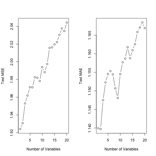
Cross-validated 10-fold subset selection produces the same answer for test MSE, but a different one for test MAE. The 10-fold CV tells us the minimum test MSE occurs with the 1-variable model. The 10-fold CV tells us the minimum test MAE occurs with the 2-variable model and has a large reduction in error with the 10-variable model. Recall, the range of our response variable is approximately 0 to 7 and our lowest root MSE is 1.396 (1-var model) and our lowest test MAE is 1.140 (2-var model) with the 10-variable model at 1.155 MAE.
coef(ff2.bestsub.total, 1)## (Intercept) monthdec
## 1.085148 1.486522coef(ff2.bestsub.total, 2)## (Intercept) monthdec temp
## 0.57120277 1.87906042 0.02684671coef(ff2.bestsub.total, 10)## (Intercept) X monthdec monthjun monthmar
## 0.211598289 0.053797867 1.860354192 -0.532651270 -0.403198781
## monthsep DMC DC temp wind
## 0.506994774 0.003148472 -0.001212802 0.031520861 0.059630087
## rain2TRUE
## -0.821049959I use the coefficients for the whole dataset to get highest accuracy for the 1 and 10 variable models.
Ok so let’s recap what we have learned about our predictors.
Two types of cross validation were used here to determine the best predictors. The first was a simple 90-10 split between the training data and the test data. Here I performed optimization on $C_p$, $R^2_a$, and $BIC$, where all gave different solutions including the 5-variable, 12-variable, and 2-variable models respectively. I then performed cross-validation with our test set where I obtained a minimum MSE & MAE with the 1-variable model (i.e. logarea ~ monthdec), but the 11-variable model and nearly as low an MAE with 0.9463533, and optimizes other diagnostics more than the 1-variable model. Then I went through a 10-fold cross-validation subset selection, which also yielded the 1-variable model. However, the 10-variable model (logarea ~ X + monthdec + monthjun + monthmar + monthsep + DMC + DC + temp + wind + rain2) had a strongly decreased MAE compared to the previous models and optimizes other diagnostics more than the 1-variable model.
So I am kind of stuck between the 10 variable model or the 11 variable model, so I will run an anova F-test.
model10 <- lm(logarea ~ X + I(month=='dec') + I(month=='jun') + I(month=='mar') + I(month=='sep') + DMC + DC + temp + wind + rain2, data = ff2Train)
model11 <- lm(logarea ~ X + I(month=='dec') + I(month=='feb') + I(month=='sep') + I(day=='tue') + DMC + DC + ISI + temp + wind + rain2, data = ff2Train)
anova(model10, model11)
## Analysis of Variance Table
##
## Model 1: logarea ~ X + I(month == "dec") + I(month == "jun") + I(month ==
## "mar") + I(month == "sep") + DMC + DC + temp + wind + rain2
## Model 2: logarea ~ X + I(month == "dec") + I(month == "feb") + I(month ==
## "sep") + I(day == "tue") + DMC + DC + ISI + temp + wind +
## rain2
## Res.Df RSS Df Sum of Sq F Pr(>F)
## 1 457 884.30
## 2 456 879.35 1 4.9517 2.5678 0.1098The ANOVA F-test indicates that there is no good reason to use the 11-variable model over the 10-variable model.
So after our diagnostics our best model is the 10-variable model: logarea ~ X + monthdec + monthjun + monthmar + monthsep + DMC + DC + temp + wind + rain2TRUE.
Just to make sure there isn’t anything odd going on with our month variables we should take a look at a visual,
plot(ff2$month, ff2$logarea)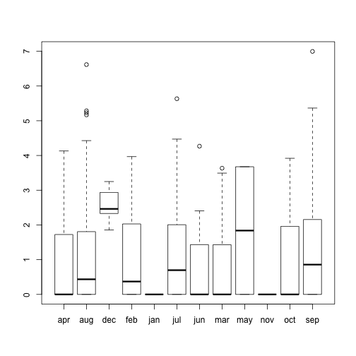
So it does seem that the September month could be included due to an outlier or a multi-day fire that was very large in area burnt each day. However, these fires still must take part in the prediction process so they will not be removed. December does not seem to be due to an outlier at all; there just seem to be a lot of medium sized fires in December. A possible reason for this could be people travelling for the holidays and then starting a forest fire.
Let’s take a look at it along with the residuals.
final.model <- lm(logarea ~ X + I(month=='dec') + I(month=='jun') + I(month=='mar') + I(month=='sep') + DMC + DC + temp + wind + rain2, data = ff2Train)
summary(final.model)
##
## Call:
## lm(formula = logarea ~ X + I(month == "dec") + I(month == "jun") +
## I(month == "mar") + I(month == "sep") + DMC + DC + temp +
## wind + rain2, data = ff2Train)
##
## Residuals:
## Min 1Q Median 3Q Max
## -1.8524 -1.0288 -0.5327 0.8570 5.2954
##
## Coefficients:
## Estimate Std. Error t value Pr(>|t|)
## (Intercept) 0.0206717 0.3872725 0.053 0.95745
## X 0.0468845 0.0280374 1.672 0.09517 .
## I(month == "dec")TRUE 2.1240498 0.6736137 3.153 0.00172 **
## I(month == "jun")TRUE -0.4664052 0.3834046 -1.216 0.22443
## I(month == "mar")TRUE -0.3444337 0.3019958 -1.141 0.25467
## I(month == "sep")TRUE 0.5239788 0.1851031 2.831 0.00485 **
## DMC 0.0033459 0.0015441 2.167 0.03076 *
## DC -0.0011847 0.0005994 -1.976 0.04872 *
## temp 0.0406331 0.0144827 2.806 0.00524 **
## wind 0.0620272 0.0390185 1.590 0.11260
## rain2TRUE -0.8036091 0.5885446 -1.365 0.17279
## ---
## Signif. codes: 0 '***' 0.001 '**' 0.01 '*' 0.05 '.' 0.1 ' ' 1
##
## Residual standard error: 1.391 on 457 degrees of freedom
## Multiple R-squared: 0.06509, Adjusted R-squared: 0.04463
## F-statistic: 3.182 on 10 and 457 DF, p-value: 0.0005814We see that our $R^2_a$ hasn’t changed much, but the model p-value has decreased significantly down to about 0.0006. Our test MAE is 1.155, which hinders our predictive power.
xyplot(rstudent(final.model) ~ fitted(final.model),
  xlab = "Fitted Values",
  ylab = "Residuals",
  panel = function(x, y, ...)
  {
    panel.grid(h = -1, v = -1)
    panel.abline(h = 0)
    panel.xyplot(x, y, ...)
  }
)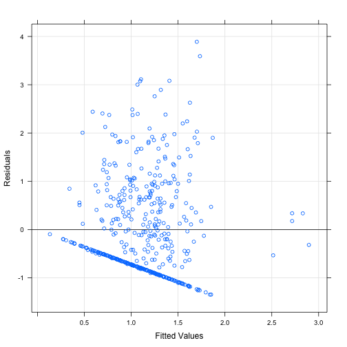
The diagonal (almost) solid line in the studentized residual plot is from the large number of 0’s in the response variable. We seem to have an issue with variance, but we have transformed this to the best of our abilities within the linear framework. Possible future work can be done with censor models and zero-inflated models.
newdata = data.frame(X=5, month="dec", DMC = 150, DC = 550, temp=15, wind = 7, rain2 = "TRUE")
predict(final.model, newdata, interval = "predict")
## fit lwr upr
## 1 2.469529 -0.7508781 5.689936Here I have a 95% prediction interval for the case where a fire occurs on a rainy/windy Tuesday in December and it is 15 degrees celcius in the middle portion of Montesinho natural park. Our interval does contain 0, which means a fire would most likely burn a small - medium radius (recall these values are exponents since we took log transform of area).
error <- fitted(final.model) - ff2Train$logarea
RMSEtrain <- sqrt(mean((error)^2))
MAEtrain <- mean(abs(error))
cat("The train RMSE is", RMSEtrain)
## The train RMSE is 1.374602cat("The train MAE is", MAEtrain)## The train MAE is 1.122505So what we see here is that the training RMSE is about 1.37 and the test RMSE was 1.39. This indicates that our model did not overfit the data, so there is still hope for our model’s predictive power.
Outliers Analysis
I obtain the studentizded deleted residuals and use the Bonferroni outlier test procedure with $\alpha$ = .01, and a Bonferroni critical value of $t(1 - \frac{\alpha}{2n}, n - p - 1)$ where $n=517$ and $p=10$. There are no outliers in the Y direction. Leverage values greater than $\frac{2p}{n}$ are considered outlying cases with regard to their X values. There are 41 outliers in the X direction.
rstu.fin <- rstudent(final.model)
rstu.fin.df <- data.frame(rstu.fin)
outy.fin <- rstu.fin > qt(1 - .01/1034, 517-11-1)
sum(outy.fin) # number of outliers in Yhii <- hatvalues(final.model)
outx.fin <- hii > 20/517
sum(outx.fin) # number of outliers in Xcat("The cases of outliers in the X direction are", names(hii[sapply(20/517, function(x) hii > x)]))## The cases of outliers in the X direction are 23 60 76 105 151 244 275 276 277 279 282 285 287 296 297 298 299 300 302 303 304 370 371 375 395 400 401 412 449 460 463 464 470 473 474 475 476 500 501 502 510The largest influence comes from case #23.
inf.fin <- cbind(dffits(final.model), dfbetas(final.model), cooks.distance(final.model))
inf.fin23 <- data.frame(inf.fin[23,])
rownames(inf.fin23) <- c("DFFITS", "DBETAS Intercept", "DBETAS X", "DBETAS December", "DBETAS June", "DBETAS March", "DBETAS September", "DBETAS DMC", "DBETAS DC", "DBETAS temp", "DBETAS wind", "DBETAS Rain", "Cook's D")
inf.fin23
## inf.fin.23...
## DFFITS -0.135341451
## DBETAS Intercept 0.044698669
## DBETAS X -0.061124837
## DBETAS December 0.014030825
## DBETAS June 0.016267770
## DBETAS March 0.024003010
## DBETAS September -0.080908361
## DBETAS DMC -0.012632041
## DBETAS DC 0.025737627
## DBETAS temp -0.013086998
## DBETAS wind -0.072849752
## DBETAS Rain 0.016281335
## Cook's D 0.001663918For this sized dataset the DBETAS and Cook’s Distance cutoff is 1, so we have no problems here.
I believe that the biggest take-away here can be seen in the estimated $\beta$ coefficients. For instance, in the variable temp we see that a 1 degree increase in temperature is associated with a multiplicative change of $e^{\beta_{temp}} = 1.03623$ in the median of area burnt. We’ve also found significance amongst the meteorological variables DMC - Duff Moisture Code (DMC), DC - Drought Code (DC), which could be useful to park rangers if they have constant access to these features. More research needs to be conducted on the occurence of forest fires in the month of December and September.