
library(dplyr)
library(ggplot2)
library(leaps)
library(knitr)
library(caret)
library(corrplot)
library(gmodels)
library(mosaic)
library(multcomp)
library(DescTools)
library(glmnet)
This data considers forest fire data from the Montesinho natural park in the Tr’as-os-Montes northeast region of Portugal. The data used in the experiments was collected from January 2000 to December 2003. The goal is to learn more about the variables involved with predicting forest fires and possibly classify new fires as big or small based on simple atmospheric indicators.
Recall the following variable descriptions,
- X - x-axis spatial coordinate within the Montesinho park map: 1 to 9
- Y - y-axis spatial coordinate within the Montesinho park map: 2 to 9
- month - month of the year: “jan” to “dec”
- day - day of the week: “mon” to “sun”
- FFMC - Fine Fuel Moisture Code (FFMC) index from the Fire Weather Index (FWI) system: 18.7 to 96.20
- DMC - Duff Moisture Code (DMC) index from the FWI system: 1.1 to 291.3
- DC - Drought Code (DC) index from the FWI system: 7.9 to 860.6
- ISI - Initial Spread Index (ISI) from the FWI system: 0.0 to 56.10
- temp - temperature in Celsius degrees: 2.2 to 33.30
- RH - relative humidity in %: 15.0 to 100
- wind - wind speed in km/h: 0.40 to 9.40
- rain2 - outside rain in mm/m2 : 0.0 to 6.4
- area - the burned area of the forest (in ha): 0.00 to 1090.84
ff <- read.csv("forestfires.csv")
ff2 <- ff %>% mutate(rain2 = as.factor(rain > 0), logarea = log(area + 1), X = as.factor(X), Y = as.factor(Y)) %>% dplyr::select(-c(rain, area))
dim(ff2)
str(ff2)
We can see that our initial dataset contains 13 variables with 517 observations.
Also recall from the simple linear regression report that we will be using the log transform of area burnt (in hectares), and we will be using rain as a factor variable (i.e. whether or not it is raining at the time of the fire).
One-Way ANOVA
In the linear model, we found that there was sufficient reason to include 4 factor levels from the ‘month’ variable. These were, December, June, March, and September. But I wonder if the difference in the means between these factor levels is simply due to chance, or is there a true difference between the population means. We will now use ANOVA to test if there is a difference between the factor level means.
We want to test the hypothesis,
\[H_0: \mu_1 = \mu_2 = \mu_3 = \mu_4\] \[H_1: not H_0\]To test this hypothesis we will look at a graph of individual fires and their log area burnt for the months in question. We also can look at a table of the means for each month and finally an ANOVA table.
month_1 <- factor(ff2$month, levels = c('dec', 'jun', 'mar', 'sep'))
xyplot(logarea ~ month_1, data = ff2, pch=19, xlab="month", ylab="log(area burnt)")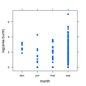
means <- aggregate(logarea ~ month_1, data = ff2, FUN=mean)
means
## month_1 logarea
## 1 dec 2.5716700
## 2 jun 0.8430907
## 3 mar 0.7725645
## 4 sep 1.2745374month.aov <- aov(logarea ~ month_1, data = ff2)
anova(month.aov)## Analysis of Variance Table
##
## Response: logarea
## Df Sum Sq Mean Sq F value Pr(>F)
## month_1 3 29.86 9.9524 5.0762 0.001987 **
## Residuals 248 486.23 1.9606
## ---
## Signif. codes: 0 '***' 0.001 '**' 0.01 '*' 0.05 '.' 0.1 ' ' 1#qf(.95, 3, 248)At the $\alpha = 0.05$ level of significance, there is sufficient reason to reject $H_0$ since our F statistic is greater than 2.641. Also, in the ANOVA table there is a p-value of 0.002, which leads us to believe there is a difference between these months, on average.
But what we have reject here is that all of the means are equal. It is possible that only one mean is different than the rest. Let’s look at a boxplot to get a better sense of the distributions.
boxplot(logarea ~ month_1, data = ff2, ylab = "log(area burnt)")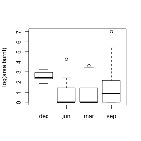
So based on this boxplot, it is likely that one month is the cause of the difference in means. But we are not certain yet. We want to check pairwise comparisons for this purpose.
TukeyHSD(month.aov)## Tukey multiple comparisons of means
## 95% family-wise confidence level
##
## Fit: aov(formula = logarea ~ month_1, data = ff2)
##
## $month_1
## diff lwr upr p adj
## jun-dec -1.72857927 -3.22155566 -0.23560288 0.0159040
## mar-dec -1.79910546 -3.10306502 -0.49514590 0.0024178
## sep-dec -1.29713261 -2.53554643 -0.05871879 0.0360751
## mar-jun -0.07052619 -1.07773570 0.93668331 0.9978862
## sep-jun 0.43144666 -0.48932979 1.35222310 0.6198340
## sep-mar 0.50197285 -0.06297076 1.06691646 0.1011988R does most of the leg work here adjusting the p-values for multiple comparisons. So we can see that all of the significant differences between pairwise comparisons involve the month of December.
Let’s now perform a nested F-test to compare June, March, and September to December.
We want to test the hypothesis,
\[H_0: \mu_1 = \frac{\mu_2 + \mu_3 + \mu_4}{3}\] \[H_1: not H_0\]ff3 <- ff2
levels(ff3$month) <- c("apr", "aug", "dec", "feb", "jan", "jul", "group", "group", "may", "nov", "oct", "group")
means2 <- aggregate(logarea ~ factor(month, levels = c("dec", "group")), data = ff3, FUN=mean)
means2## factor(month, levels = c("dec", "group")) logarea
## 1 dec 2.571670
## 2 group 1.132804month.aov2 <- aov(logarea ~ factor(month, levels = c("dec", "group")), data = ff3)
anova(month.aov2)## Analysis of Variance Table
##
## Response: logarea
## Df Sum Sq Mean Sq F value
## factor(month, levels = c("dec", "group")) 1 17.97 17.9675 9.0177
## Residuals 250 498.12 1.9925
## Pr(>F)
## factor(month, levels = c("dec", "group")) 0.002945 **
## Residuals
## ---
## Signif. codes: 0 '***' 0.001 '**' 0.01 '*' 0.05 '.' 0.1 ' ' 1The ANOVA table shows that the nested F-test rejects $H_0$ and suggests that there is a difference between the grouped months on average compared with December. So now we want to know, does December have an affect on log(area burnt)? To figure this out we will utilize linear contrasts.
lm1 = lm(logarea ~ month_1, data = ff2); coef(lm1)## (Intercept) month_1jun month_1mar month_1sep
## 2.571670 -1.728579 -1.799105 -1.297133december = rbind('December' = c(-1, 1/3, 1/3, 1/3))
september = rbind('September' = c(1/3, 1/3, 1/3, -1))
cntrsts = rbind('December' = c(-1, 1/3, 1/3, 1/3),
'September' = c(1/3, 1/3, 1/3, -1))
summary(glht(month.aov, linfct=mcp(month_1=cntrsts),
alternative="greater"), test=adjusted("none"))##
## Simultaneous Tests for General Linear Hypotheses
##
## Multiple Comparisons of Means: User-defined Contrasts
##
##
## Fit: aov(formula = logarea ~ month_1, data = ff2)
##
## Linear Hypotheses:
## Estimate Std. Error t value Pr(>t)
## December <= 0 -1.6083 0.4858 -3.311 0.999
## September <= 0 0.1212 0.2290 0.529 0.299
## (Adjusted p values reported -- none method)ScheffeTest(month.aov, which="month_1", contrasts=t(cntrsts))##
## Posthoc multiple comparisons of means : Scheffe Test
## 95% family-wise confidence level
##
## $month_1
## diff lwr.ci upr.ci pval
## jun,mar,sep-dec -1.6082724 -2.9755691 -0.2409758 0.0132 *
## dec,jun,mar-sep 0.1212377 -0.5234158 0.7658912 0.9636
##
## ---
## Signif. codes: 0 '***' 0.001 '**' 0.01 '*' 0.05 '.' 0.1 ' ' 1We can be 95% confident that the population mean averaged from the factor level December is $e^{-2.976}$ to $e^{-0.241}$ lower than that of the other months.
We can be 95% confident that the population mean averaged from the factor level September is $e^{-0.523}$ to $e^{0.766}$ greater than that of the other months.
The Scheffe multiple comparisons procedure was employed here as we looked at the treatment means $\mu_{i.}$ in the linear contrasts.
I’m also interested to see if there is a significant difference between the mean areas burnt of the days of the week.
We want to test the hypothesis,
\[H_0: \mu_1 = \mu_2 = \mu_3 = \mu_4 = \mu_5 = \mu_6 = \mu_7\] \[H_1: not H_0\]Again, to test this hypothesis we will look at a graph of individual fires and their log area burnt for the days in question. We will also look at a table of the means for each day and the ANOVA table.
xyplot(logarea ~ day, data = ff2, pch=19, xlab="day", ylab="log(area burnt)")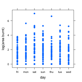
aggregate(logarea ~ day, data = ff2, FUN=mean)## day logarea
## 1 fri 0.9697708
## 2 mon 1.0899676
## 3 sat 1.2263961
## 4 sun 1.1240928
## 5 thu 1.0262667
## 6 tue 1.2307187
## 7 wed 1.1136639anova(aov(logarea ~ day, data = ff2))## Analysis of Variance Table
##
## Response: logarea
## Df Sum Sq Mean Sq F value Pr(>F)
## day 6 4.22 0.7031 0.3568 0.9059
## Residuals 510 1004.88 1.9704#qf(.95, 6, 510)Our F-statistic is not greater than the corresponding F-value at an $\alpha = 0.05$ level of significance, so there is not sufficient reason to reject the idea that there is a difference between the days of the week, on average.
Two-Way ANOVA
We can look at the additivity and interaction between two factor variables, month and vertical position (Y).
par(mfrow=c(1,3))
plot(logarea ~ month + Y, data = ff2)
with(ff2, interaction.plot(month, Y, logarea))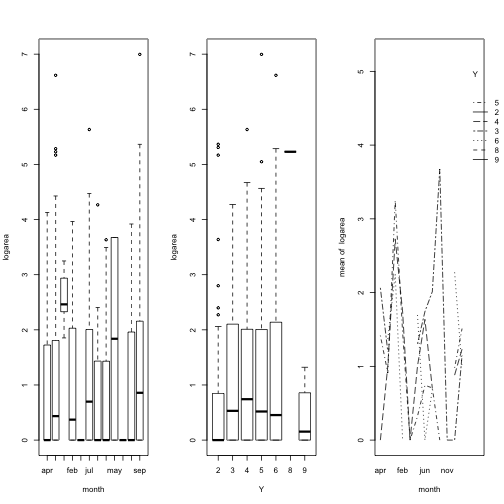
This shows slight evidence of nonadditivity and could be more than simple natrual variation. However, we will test the significance of the interaction to be sure,
monthday.aov <- aov(logarea ~ month*Y, data = ff2)
anova(monthday.aov)
## Analysis of Variance Table
##
## Response: logarea
## Df Sum Sq Mean Sq F value Pr(>F)
## month 11 37.37 3.3970 1.7887 0.05334 .
## Y 6 25.24 4.2073 2.2154 0.04052 *
## month:Y 30 55.81 1.8604 0.9796 0.49948
## Residuals 469 890.68 1.8991
## ---
## Signif. codes: 0 '***' 0.001 '**' 0.01 '*' 0.05 '.' 0.1 ' ' 1plot(monthday.aov$fitted, rstudent(monthday.aov), xlab="Fitted Raw", ylab="Student Residuals", pch=19)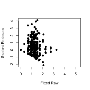
The ANOVA table indicated that the interaction term is not significant so we will only look at additive effects.
monthday2.aov <- aov(logarea ~ month + Y, data = ff2)
anova(monthday2.aov)
## Analysis of Variance Table
##
## Response: logarea
## Df Sum Sq Mean Sq F value Pr(>F)
## month 11 37.37 3.3970 1.7909 0.05277 .
## Y 6 25.24 4.2073 2.2181 0.04016 *
## Residuals 499 946.49 1.8968
## ---
## Signif. codes: 0 '***' 0.001 '**' 0.01 '*' 0.05 '.' 0.1 ' ' 1The data certainly seem more consistent with the additive model.
ff2$resid = predict(aov(logarea ~ month + Y, data = ff2))
par(mfrow=c(1,2))
plot(aov(logarea ~ month + Y, data = ff2), which=1)
plot(aov(logarea ~ month + Y, data = ff2), which=4)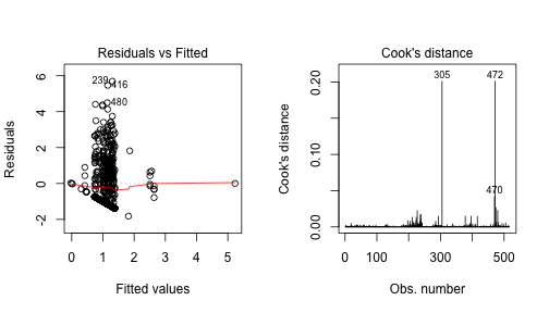
histogram(~ resid, type='density', density=TRUE, data=ff2)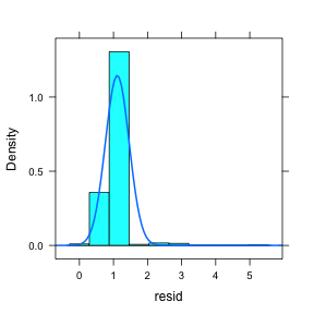
These figures indicate that the normality and linearity assumptions seems to be a problem. The equality of variance assumption seems to be broken as well, yielding a fatal error for my machine. The cook’s distance plot shows some very influential outliers with the additive model. Here they are below,
ff2[c(305, 470, 472),]## X Y month day FFMC DMC DC ISI temp RH wind rain2 logarea
## 305 6 5 may sat 85.1 28.0 113.8 3.5 11.3 94 4.9 FALSE 0.000000
## 470 6 3 apr sun 91.0 14.6 25.6 12.3 13.7 33 9.4 FALSE 4.129229
## 472 4 3 may fri 89.6 25.4 73.7 5.7 18.0 40 4.0 FALSE 3.675794
## resid
## 305 1.818040
## 470 1.137743
## 472 1.857754Logistic Regression
The biggest problem throughout this study has been the problem of censored data. The researchers decided that if a fire was less than 0.1 hectares in area burnt, they would mark this down as a fire, but with area equal to zero. Now I will attempt to erase this difficulty in skewed response by changing the problem slightly to a classification problem. Now I will attempt to predict whether the fire is a ‘big’ fire. Big fires will be denoted by the log(area burnt) > 3.
For feature selection we will use a lasso with cross-validation.
ffclass <- ff2 %>% mutate(bigfire = logarea > 3) %>% dplyr::select(-logarea)
ffclass$bigfire <- as.factor(ffclass$bigfire)
X <- ffclass$X; X <- as.factor(X)
Y <- ffclass$Y; Y <- as.factor(Y)
month <- ffclass$month; month <- as.factor(month)
day <- ffclass$day; day <- as.factor(day)
FFMC <- ffclass$FFMC
DMC <- ffclass$DMC
DC <- ffclass$DC
ISI <- ffclass$ISI
temp <- ffclass$temp
RH <- ffclass$RH
wind <- ffclass$wind
rain2 <- ffclass$rain2; rain2 <- as.factor(rain2)
bigfire <- ffclass$bigfire
xfactors <- model.matrix(bigfire ~ X + Y + month + day + rain2)[,-1]
x <- as.matrix(data.frame(FFMC, DMC, DC, ISI, temp, RH, wind, xfactors))
glmmod <- glmnet(x, y=as.factor(bigfire), alpha=1, family='binomial')
plot(glmmod,xvar="lambda")
grid()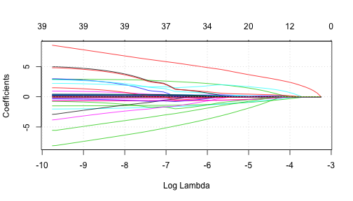
coef(glmmod)[,10]## (Intercept) FFMC DMC DC ISI
## -2.137685872 0.000000000 0.000000000 0.000000000 0.000000000
## temp RH wind X2 X3
## 0.000000000 -0.001484071 0.033531851 -0.069033251 -0.375203944
## X4 X5 X6 X7 X8
## 0.063193725 -0.205011497 0.000000000 0.000000000 0.000000000
## X9 Y3 Y4 Y5 Y6
## 0.146788302 0.012437035 0.000000000 0.000000000 0.000000000
## Y8 Y9 monthaug monthdec monthfeb
## 2.518580684 0.000000000 0.000000000 0.000000000 0.000000000
## monthjan monthjul monthjun monthmar monthmay
## 0.000000000 0.000000000 0.000000000 0.000000000 0.838989996
## monthnov monthoct monthsep daymon daysat
## 0.000000000 0.000000000 0.200451646 0.000000000 0.000000000
## daysun daythu daytue daywed rain2TRUE
## 0.000000000 -0.063985812 0.000000000 0.000000000 0.000000000cv.glmmod <- cv.glmnet(x, y=bigfire, alpha=1, family='binomial')
plot(cv.glmmod)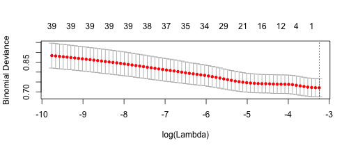
best_lambda <- cv.glmmod$lambda.min
cat("The best lambda value using cross validation is", best_lambda)
## The best lambda value using cross validation is 0.03891355So cross validated lasso tells us that the optimal lambda value is the one that corresponds to the model with only the intercept term. So this is not very helpful. But I will instead use the variables with non-zero coefficients from the glmnet lasso.
set.seed(511)
glm.fit <- glm(bigfire ~ RH + wind + I(X=='2') + I(X=='3') + I(X=='4') + I(X=='5') + I(X=='9') + I(Y=='3') + I(month=='dec') + I(month=='may') + I(month=='sep') + I(day=='thu'), data = ffclass, family = binomial)
summary(glm.fit)
##
## Call:
## glm(formula = bigfire ~ RH + wind + I(X == "2") + I(X == "3") +
## I(X == "4") + I(X == "5") + I(X == "9") + I(Y == "3") + I(month ==
## "dec") + I(month == "may") + I(month == "sep") + I(day ==
## "thu"), family = binomial, data = ffclass)
##
## Deviance Residuals:
## Min 1Q Median 3Q Max
## -0.9678 -0.5519 -0.4227 -0.2773 2.6343
##
## Coefficients:
## Estimate Std. Error z value Pr(>|z|)
## (Intercept) -2.054593 0.582963 -3.524 0.000424 ***
## RH -0.016172 0.009476 -1.707 0.087882 .
## wind 0.165166 0.084576 1.953 0.050835 .
## I(X == "2")TRUE -0.700534 0.509485 -1.375 0.169136
## I(X == "3")TRUE -1.476478 0.751438 -1.965 0.049429 *
## I(X == "4")TRUE 0.150352 0.354701 0.424 0.671650
## I(X == "5")TRUE -1.563292 1.040311 -1.503 0.132912
## I(X == "9")TRUE 1.026058 0.717094 1.431 0.152471
## I(Y == "3")TRUE 0.155498 0.388511 0.400 0.688979
## I(month == "dec")TRUE 0.177348 0.930324 0.191 0.848815
## I(month == "may")TRUE 2.250212 1.503902 1.496 0.134589
## I(month == "sep")TRUE 0.647498 0.303800 2.131 0.033062 *
## I(day == "thu")TRUE -0.895065 0.552355 -1.620 0.105135
## ---
## Signif. codes: 0 '***' 0.001 '**' 0.01 '*' 0.05 '.' 0.1 ' ' 1
##
## (Dispersion parameter for binomial family taken to be 1)
##
## Null deviance: 371.19 on 516 degrees of freedom
## Residual deviance: 343.38 on 504 degrees of freedom
## AIC: 369.38
##
## Number of Fisher Scoring iterations: 6glm.probs = predict(glm.fit, type = "response")
glm.probs <- data.frame(glm.probs)glm.pred=rep("FALSE", 517)
glm.pred[glm.probs > .15] = "TRUE"
table(glm.pred, ffclass$bigfire,dnn=c("Prediction","Truth"))## Truth
## Prediction FALSE TRUE
## FALSE 338 27
## TRUE 119 33hist(predict(glm.fit, type = "response"), xlab = "Individual Probabilities of Big Fire", main = NULL)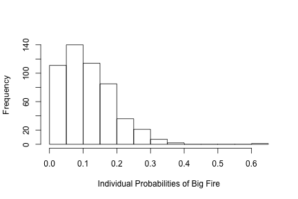
cat("The training error rate is", 100 - 100*mean(glm.pred == ffclass$bigfire), "%")## The training error rate is 28.23985 %So we find significance in the month of September (a positive relationship with log area burnt) and with the horizontal map position of 3 (a negative relationship with log area burnt) and wind (a positive relationship with log area burnt).
We are willing to allow our model to predict there is a big fire when it’s actually a small fire because we really wouldn’t want the model to miss a big fire. In other words, we will allow some false positives in order to reduce the number of false negatives.
Summary
This model has confirmed our previous model’s intuition that September has a significant predictive relationship with area burnt in these firest fires. The logistic model seems to have a stronger positive relationship with wind and area burnt than the previous linear model. ANOVA told us that there is something intrinsically different about the month of December in relation to area burnt. This could be due to people on holiday starting fires, since most forest fires are started by humans (thanks Smokey the Bear). With the horizontal map position of 3 being a strong negitive predictor of area burnt, after some research I do not have a good explanation for why this might be.
While the linear model found a significant relationship between Duff Moisture Code (DMC), Drought Code (DC), temperature and area burnt, the logistic regression did not. And while the logistic regression found significance in wind speed, the linear model did not. In my opinion, the logistic regression is mroe reliable as it was not affected by the cencorship problem described previously.
Beyond the Model, Looking Into Logistic Regression
We will now reduce the problem down to two predictors and the classifier label (bigfire) so that we can take a closer look at what R is doing under the hood with logistic regression.
The big difference between the previous linear regression and now the logistic regression is the response variable is now binary. In other words, the y-variable (dependent variable) went from being continuous to just being either 0 or 1.
So if we set our 0 and 1 appropriately, 1 - big fire and 0 - small fire, we want to obtain probabilities that the response takes on a value of 1. The logistic function (or sigmoid function) is perfect for our purposes because its behavior allows us to set a hypothesis between 0 and 1. If we state our hypothesis, $h(x)$ as the probability that y takes a value of 1, $h(x)$ is a function of some paramater $\theta$ and our data $x$, where $h(x) = g(\theta^T x)$ and $g(z)$ is the sigmoid function $\frac{1}{1 + e^{-z}}$.
So when will our hypothesis make a prediction of 1 and when will it make a prediction of 0? The answer to this question has to do with the decision boundary.
We can say that the model will predict 1 if our hypothesis is greater than or equal to some probability, say 0.5. And when it is less than 0.5 the model predicts 0. So if our hypothesis is just the sigmoid function evaluated at $\theta^T x$ then we can say the model will predict 1 when $\theta^T x \geq 0$. But how do we estimate the parameter(s)? As you might expect, finding the parameters necessary for the model is an optimization problem.
\[J(\theta) = \dfrac{1}{m} \sum_{i=1}^m \text{Cost}(h_\theta(x^{(i)}),y^{(i)})\] \[\text{Cost}(h_\theta(x),y) = -\log(h_\theta(x)), \text{if y = 1}\] \[\text{Cost}(h_\theta(x),y) = -\log(1-h_\theta(x)), \text{if y = 0}\]So this is very useful because the more the hypothesis is off from y, the larger the cost function output. And if the hypothesis is equal to y, the cost is 0. This guarantees the convexity of $J(\theta)$ and that we can obtain a proper minimization.
However, this cost function can be joined in the form,
\[\text{Cost}(h_\theta(x),y) = - y \log(h_\theta(x)) - (1 - y) \log(1 - h_\theta(x))\]and $J(\theta)$ becomes
\[J(\theta) = - \frac{1}{m} \sum_{i=1}^m [y^{(i)}\log (h_\theta (x^{(i)})) + (1 - y^{(i)})\log (1 - h_\theta(x^{(i)}))]\]or in vector format,
\[J\left(\theta\right) = -\frac{1}{m}\left(\log\left(g\left(X\theta\right)\right)^{T}y+\log\left(1-g\left(X\theta\right)\right)^{T}\left(1-y\right)\right)\]Now we can implement gradient descent.
We can see this implemented with MATLAB and two of the continuous predictors Duff Moisture Code (DMC) and Drought Code (DC). Using these two predictors allows us to visualize the data and the decision boundary, as seen in the figures below.
%%MATLAB
%% Data
clear ; close all; clc

data = load('ffclass.txt');
X = data(:, [1, 2]); y = data(:, 3);

fprintf(['Plotting data with + indicating (y = 1) examples and o ' ...
         'indicating (y = 0) examples.\n']);

plotData(X, y);

% Put some labels
hold on;
% Labels and Legend
xlabel('Duff Moisture Code (DMC)')
ylabel('Drought Code (DC)')

% Specified in plot order
legend('Big Fire', 'Small Fire')
hold off;

pause;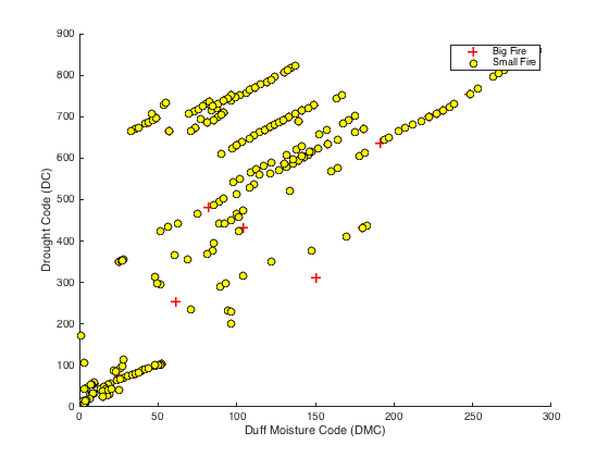
%% Cost and Gradient

%  Matrix for our data
[m, n] = size(X);

% Intercept term
X = [ones(m, 1) X];

% Fitting parameters
initial_theta = zeros(n + 1, 1);

% Initial cost and gradient
[cost, grad] = costFunction(initial_theta, X, y);

fprintf('Cost at initial theta (zeros): %f\n', cost);
fprintf('Gradient at initial theta (zeros): \n');
fprintf(' %f \n', grad);

pause;
## Cost at initial theta (zeros): 0.693147
## Gradient at initial theta (zeros):
## 0.383946
## 42.411605
## 208.871567
## Local minimum possible.%% Optimization with fminunc
% Set options for fminunc
options = optimset('GradObj', 'on', 'MaxIter', 400);
% Run fminunc to obtain the optimal theta
% This function will return theta and the cost
[theta, cost] = ...
fminunc(@(t)(costFunction(t, X, y)), initial_theta, options);
% Print theta to screen
fprintf('Cost at theta found by fminunc: %f\n', cost);
fprintf('theta: \n');
fprintf(' %f \n', theta);
% Plot Boundary
plotDecisionBoundary(theta, X, y);
% Put some labels
hold on;
% Labels and Legend
xlabel('Duff Moisture Code (DMC)')
ylabel('Drought Code (DC)')
% Specified in plot order
legend('Big Fire', 'Small Fire')
hold off;
pause;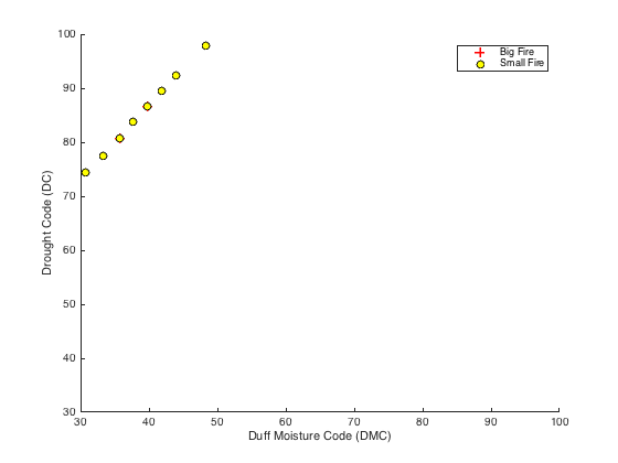
##   Cost at theta found by fminunc: 0.358790
## theta:
##  -2.123344
##  -0.000557
##  0.000291
##  For a day with scores DMC = 110 and DC = 540, we predict a big fire probability of 0.116324
%% Prediction
prob = sigmoid([1 110 540] * theta);
fprintf(['For a day with scores DMC = 110 and DC = 540, we predict a big fire ' ...
'probability of %f\n\n'], prob);
% Accuracy on our training set
p = predict(theta, X);
%p = 0;
fprintf('Train Accuracy: %f\n', mean(double(p == y)) * 100);
pause;## Train Accuracy: 88.394584