Hidden Markov Model Simulation

HMM Simulation

Without having formally worked in Hidden Markov Models before, this is my attempt at reinterpreting a well known solution in the computational biology domain. I read an article in Nature magazine by Sean R Eddy, which will serve as a perfect problem for me to attempt an HMM simulation akin to the Eddy example. I encourage you to brief yourself on the article before continuing here. Don’t worry, it’s very short.

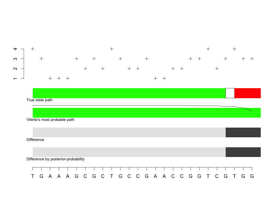
We simulate a string of length 26 (as in the Eddy study) and determine the probability of that string given the structure while inferring the hidden state path. The model is probably looking for an even number of A,C,G,T for the beginning and once there’s too many G’s it marks it as a “5SS”. This is because the “5SS” state has very high probability in G and “exon” has even probability throughout. That is why we see the change from green to red occur on a G observation (seen below).

require(HMM)
 nSim = 26
 States = c("S","exon", "5SS", "intron", "N")
 Symbols = LETTERS[c(1,3,7,20)]
 transitions = matrix(c(0,1, 0, 0, 0, 0, 0.9, 0.1, 0, 0,0,0,0,1,0,0,0,0,0.9,0.1,0,0,0,0,1), c(length(States), length(States)), byrow = TRUE)
 row0 <- c(0,0,0,0)
 row1 <- c(1/4, 1/4, 1/4, 1/4)
 row2 <- c(0.05, 0, 0.95, 0)
 row3 <- c(0.4,0.1,0.1,0.4)
 row4 <- c(0,0,0,0)
 set.seed(513)
 emissions = matrix(c(row0,row1,row2,row3,row4), nrow=5, ncol=4, byrow = TRUE)
 hmm = initHMM(States, Symbols, transProbs = transitions, emissionProbs = emissions)
 sim = simHMM(hmm, 26)
 vit = viterbi(hmm, sim$observation)
 f = forward(hmm, sim$observation)
 b = backward(hmm, sim$observation)
 i <- f[2, nSim]
 j <- f[3, nSim]
 probObservations = (i + log(1 + exp(j - i)))
 posterior = exp((f + b) - probObservations)
 x = list(hmm = hmm, sim = sim, vit = vit, posterior = posterior)
 
plot(as.numeric(factor(x$sim$observation)), ylim = c(-7.5, 6), pch=3, ylab = ylb, xlab = "", bty = "n", xaxt = "n", yaxt = "n"); axis(1, at=seq_along(x$sim$observation), labels=x$sim$observation)
axis(2, at = 1:4)

# Simulating (truth) #
 text(0.3, -1.2, adj = 0, cex = 0.8, col = "black", "True state path")
 for (i in 1:nSim) {
    if (x$sim$states[i] == "exon")
        rect(i, -1, i + 1, 0, col = "green", border = NA)
   else if (x$sim$states[i] == "5SS")
     rect(i, -1, i + 1, 0, col = "white")
    else rect(i, -1, i + 1, 0, col = "red", border = NA)
   }
# Inference and Viterbi algorithm: finding the most probable path #
text(0.3, -3.2, adj = 0, cex = 0.8, col = "black", "Viterbi's most probable path")
for (i in 1:nSim) {
    if (x$vit[i] == "exon")
        rect(i, -3, i + 1, -2, col = "green", border = NA)
  else if (x$sim$states[i] == "5SS")
    rect(i, -1, i + 1, 0, col = "white")
    else rect(i, -3, i + 1, -2, col = "red", border = NA)
}
# Differences:
text(0.3, -5.2, adj = 0, cex = 0.8, col = "black", "Difference")
differing = !(x$sim$states == x$vit)
for (i in 1:nSim) {
    if (differing[i])
        rect(i, -5, i + 1, -4, col = rgb(0.3, 0.3, 0.3),
            border = NA)
    else rect(i, -5, i + 1, -4, col = rgb(0.9, 0.9, 0.9),
        border = NA)
       }
 
 points(x$posterior[2, ] - 3, type = "l")
 # Difference with classification by posterior-probability:
 text(0.3, -7.2, adj = 0, cex = 0.8, col = "black", "Difference by posterior-probability")
 differing = !(x$sim$states == x$vit)
 for (i in 1:nSim) {
    if (posterior[2, i] > 0.5) {
        if (x$sim$states[i] == "exon")
            rect(i, -7, i + 1, -6, col = rgb(0.9, 0.9, 0.9),
              border = NA)
        else rect(i, -7, i + 1, -6, col = rgb(0.3, 0.3, 0.3),
            border = NA)
     }
     else {
         if (x$sim$states[i] == "intron")
             rect(i, -7, i + 1, -6, col = rgb(0.9, 0.9, 0.9),
               border = NA)
         else rect(i, -7, i + 1, -6, col = rgb(0.3, 0.3, 0.3),
            border = NA)
      }
    }

This code generates the same type of model as the Eddy article. The top portion indicates the 26 simulated observation sequence. The true state path is green when the state is “exon” and white when it becomes “5SS” and then red once it becomes “intron”. I guess Viterbi can’t pick up on the subtlety of the extra G that creates the “5SS” state, the algorithm believes we remained in “exon” for the entirety. The viterbi moving average line does seem to indicate a possibly change in state towards the end of the sequence, but it was not represented in the final output. We then observe the difference and the difference by posterior probability between Viterbi and the true state path. The difference is like a density of false positives and represents the errors in the model. The posterior difference uses forward - backward algorithm which is a Bayesian technique, which is why we call it the posterior difference.

With so few states and observations we could probably just enumerate all possible state sequences and find the one with the highest probability, but this is not scalable. We could also consider a more unsupervised approach to learning the parameters. We could use an iterative process like EM algorithm to find the MLE.

A Look at the Evaluation and Decoding Algorithms

Let’s suppose we have an HMM structure like model with N observations $(y = y_1:N)$, but there is a way we know the value of the hidden states $(x)$ in the chain as well as the observables. In this case we could easily calculate the likelihood

If we do not observe the hidden states, then,

Because we have structure we can exploit this with a dynamic programming algorithm for calculating the likelihood.

For evaluation, forward algorithm is used to calculate what the probability is of the observed sequence. The algorithm computes the probability, $p(x_k, y_{1:k})$. Using the Markov property, i.e. the conditional probability distribution of future states of the process depends only upon the present state, not on the sequence of events that preceded it, we can see that \(p(x_k, y_{1:k}) = \sum_{x_{k-1}}p(x_k,x_{k-1},y_{1:k})\) when summing over all possibly values of $x_{k-1}$. This leads us to \(\sum_{x_{k-1}}p(y_k|x_k,x_{k-1},y_{1:k-1})p(x_k|x_{k-1},y_{1:k-1})p(x_{k-1}|y_{1:k-1})p(y_{1:k-1})\), where \(p(x_{k-1}|y_{1:k-1})p(y_{1:k-1})=p(x_{k-1},y_{1:k-1})\).

Now independence can be applied to the first term in the summation \(p(y_k|x_k,x_{k-1},y_{1:k-1})\) since we can just say this equates to $p(y_k|x_k)$, and the second term \(p(x_k|x_{k-1},y_{1:k-1})\) can be simplified to \(p(x_k|x_{k-1})\).
Which leaves us with \(p(x_k, y_{1:k}) = \sum_{x_{k-1}}p(y_k|x_k)p(x_k|x_{k-1})p(x_{k-1},y_{1:k-1}) = \alpha_k(x_k)\).

As we just saw, forward algorithm computes the probability \(p(x_k,y_{1:k})\).
Backward algorithm instead computes the joint distributions of \(p(y_{k+1:n}|x_k)\). Backward works recursively. While the methods are different, Forward and the Backward algorithm can be used to determine the probability of a sequence.

Viterbi algorithm deals with the decoding problem (given a sequence and a model, what is the most likely sequence of states that produced the sequence), while forward algorithm deals with the evaluation problem (what is the probability that a particular sequence is produced by a particular model).

Posterior decoding makes use of the forward and backward algorithms. The goal is to determine the path through the hidden markov model that corresponds to true labeling of the data. Instead of determining the most probable path (as in Viterbi), posterior decoding determines, independently, for every symbol $O_t$ the most probable state using,

This method is based on the posterior probability of emitting $X$ from state $k$ when the emitted sequence is known. This is why it is called posterior decoding.

this is saying that the probability of being in state $k$ when $X$ is emitted, is equivalent to the emitting $x_1…x_{i-1}$ over any path, entering $k$, emitting $x_i$, and then emitting $x_{i+1}, x_{i+2}, …, x_N$ over any path. The first term is just $\alpha_i(k)$ and we calculate the second term with the backward algorithm, which is also used to calculate $P(x)$.

The difference between Viterbi and posterior decoding is that in position $i$, the Viterbi algorithm calculates,

However, there is not one statement that says one is better than the other. Much of this depends on how likely the Viterbi optimal path is. If the optimal path is only marginally better than alternatives, posterior decoding may be the better choice. Posterior decoding is better in instances when you want to take into account all possible paths.

Learning in Graphical Models

The Expectation and Maximization (EM) algorithm is an efficient iterative procedure to compute the Maximum Likelihood Estimate (MLE) or in some cases a Maximum A-Posteriori estimate (MAP) in the case we have missing data. In an HMM, hidden variables are considered missing. So EM is used here for parameter estimation.

To handle the missing data, we kind of pretend that we have data and structure to calculate the maximum likelihood estimators for the $x$’s. Given a random vector $y = {y_1, y_2, …, y_n}$ of observed variables we also have some $x = {x_1, x_2, …, x_n}$ that we don’t know. So we have $y$ and $x$ and we calculate the density given the parameters and the distribution and parameters are associated to the concatenation of the observables and the non-observed. The first thing we try to do is estimate the non-observed. This is the E-algorithm and gives us the $\hat{x}_i$’s.

So the $(y,x)$ has a joint distribution whose density is indexed by an n-dimensional parameter $\theta$. We want to compute the MLE of $\theta$ based on $y$. And the parameters will be estimated from the $y$’s and the structure.

So we want to maximize the log-likelihood funtion of $y$,

But we can only compute the log-likelihood of the observed data and then we use this to iteratively maximize the log-likelihood of the hidden portion,

To iteratively maximize the log-likelihood of the hidden portion,

wher $y$ is the $y_{obs}$ and the $x$’s.

So we are using the observables to estimate the unobserved.

In the expectation, the E-step, the missing data are estimated given the observed data and current estimate of the model parameters. In the M-step we assume that we know the missing data.