
I’m finally beginning a Kaggle competition of my own, Give Me Some Credit. I’ve decided for my first Kaggle I will try an already completed competition and see where I would’ve placed if the competition was in session. Then maybe later I will try a live one. Also, I will update my progress in multiple posts. This first post consists of dealing with the missing data using data imputation methods.
library(ggplot2)
library(lattice)
Models can not be evaluated on missing data without some processing. So if we are given a dataset with NA values, we must develop a technique to either repeal or replace them. In some cases we may just remove the NA values. But this is not always the best method. If we just remove the missing values, we can cause more variable estimates, or even worse we could cause biased estimates. Here we look at the option to replace the NA values. One benefit to replacing the NA values is that they may contain important information. We want to deal with the missing values in a way that causes minimum harm to our inference or prediction. The missing values can be missing at random or not at random. If they are missing at random there is no pattern to the way they are missing from the variable and no pattern to how they are missing compared to other variables. The other possibility is that the missing values have some pattern and are missing due to a systematic issue with data collection.
One of the simplest ways of imputing for missing values is just to impute the mean of that variable across the non-missing values. Issues with this method are that it understates variability in the variable. This method is also not making any attempt to obtain the associations between the variables.
Another method of imputing for the missing values is to do regression-based imputation, which is the method described below in R. We have a dataset from the Give me Some Credit Kaggle competition where the purpose is to predict whether or not someone will default on their credit, or in terms of the data: predict a binary response SeriousDlqin2yrs.
Train <- read.csv('cs-training.csv', header=TRUE,comment.char="")
Train$X <- NULL # Removes redundant indexing

set.seed(890522)
o<-order(runif(dim(Train)[1])) # Create index to randomly subset data

SeriousDlqin2yrs <- Train$SeriousDlqin2yrs[o[1:(.2*(dim(Train)[1]))]]
Train$SeriousDlqin2yrs <- NULL

N_var <- length(colnames(Train)) # Number of variables
N_obs <- length(Train$age) # Number of Observations
Test <- read.csv('cs-test.csv', header=TRUE, comment.char="")
Test$X <- NULL # Removes redundant indexing
Test$SeriousDlqin2yrs <- NULL # Removes redundant indexing

credit.train <- Train[o[1:(.2*(dim(Train)[1]))],]
credit.pred <- Train[o[(.2*(dim(Train)[1])+1):(.25*(dim(Train)[1]))],]
Below is a bar chart describing the number of NA values for each variable. We can see that MonthlyIncome has the most missing values and NumberOfDependents has missing values and the remaining variables do not. However, the DebtRatio variable contains innacurate information so we will also do regression imputation on these values.
train_na <- as.data.frame(sapply(credit.train, function(x) sum(is.na(x))))
train_na <- data.frame(names = row.names(train_na), count = train_na[,1])

barchart(as.factor(names) ~ count, data = train_na, title = "Number of NA counts per variable")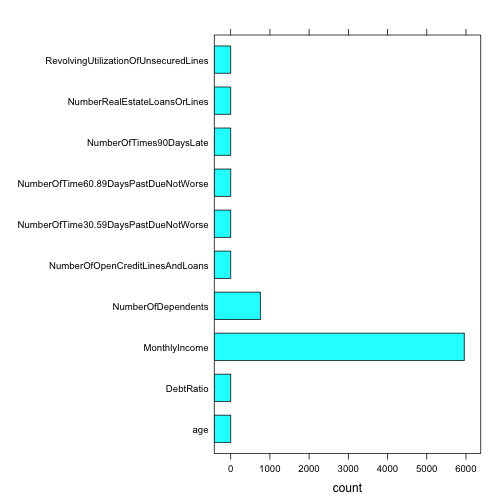
We take the data frame, do linear regression to solve for the variable in question, and then update the values in the data frame. Much like a Gibbs sampler, we hope that running this repeatedly will cause us to converge to a better value for Monthly Income, Debt Ratio, and Number of Dependents than, say, the mean of the data set.
Update_MI <- function(df,index) {
  # Updates 0 and NA values of Monthly Income
  #
  # Args:
  #   df: data frame of observations
  #
  # Returns:
  #   dataframe w/ updated values
  LinReg <- lm(MonthlyIncome ~ .,df) # Performs linear regression for Monthly Income using all other variales
  df$MonthlyIncome[index] <- predict(LinReg,df[index,]) # Imputes for Monthly Income
  print(paste("MI: ",df$MonthlyIncome[index[1]]),sep="") # Check for convergence
  return(df)
}

Update_NoD <- function(df,index) {
  # Updates NA values of Number of Dependents
  #
  # Args:
  #   df: data frame of observations
  #
  # Returns:
  #   dataframe w/ updated values
  LinReg <- lm(NumberOfDependents ~ .,df) # Performs linear regression for Monthly Income using all other variales
  df$NumberOfDependents[index] <- predict(LinReg,df[index,]) # Imputes for Number of Dependents
  print(paste("NoD: ",df$NumberOfDependents[index[1]]),sep="") # Check for convergence
  return(df)
}

Update_DR <- function(df,index) {
  # Updates Debt Ratio for Monthly Income = 0 or NA
  #
  # Args:
  #   df: data frame of observations
  #
  # Returns:
  #   dataframe w/ updated values
  LinReg <- lm(DebtRatio ~ .,df) # Performs linear regression for Debt Ratio using all other variales
  df$DebtRatio[index] <- predict(LinReg,df[index,]) # Imputes for Debt Ratio
  print(paste("DR: ",df$DebtRatio[index[1]]),sep="") # Check for convergence
  return(df)
}
Impute <- function(df) {
# Imputes NA values in the data frame using linear regression
#
# Args:
# df: data frame of observations
#
# Returns:
# data frame with imputed values for Monthly Income, Debt Ratio, and Number of Dependents
na.NoD.index <- which(is.na(df$NumberOfDependents)) # Observations with Number of Dependents = NA
na.MI.index <- which(is.na(df$MonthlyIncome)) # Observations with Monthly Income = NA
zero.MI.index <- which(df$MonthlyIncome == 0) # Observations with Monthly Income = 0
zero.na.MI.index <- sort(c(na.MI.index,zero.MI.index)) # Observations with Monthly Income = 0 or NA
Debt_Hold <- df$DebtRatio[zero.na.MI.index] # Stores Debt Values where Debt Ratio could not be calculated
df$DebtRatio[zero.na.MI.index] <- NA # Replaces Debt Values with NA
mean_NoD <- mean(df$NumberOfDependents,na.rm=TRUE) # Mean Number of Dependents
mean_DR <- mean(df$DebtRatio,na.rm=TRUE) # Mean Debt Ratio
mean_MI <- mean(df$MonthlyIncome,na.rm=TRUE) # Mean Monthly Income
df$DebtRatio[zero.na.MI.index] <- mean_DR # Insert Mean Number of Dependents as init for Observations with Monthly Income = 0 or NA
df$NumberOfDependents[na.NoD.index] <- mean_NoD # Insert Mean Number of Dependents as init for Observations with NoD = NA
# Imputation
for(i in 1:20) {
df <- Update_MI(df,zero.na.MI.index)
df <- Update_NoD(df,na.NoD.index)
df <- Update_DR(df,zero.na.MI.index)
}
df$DebtRatio[zero.na.MI.index] <- Debt_Hold / df$MonthlyIncome[zero.na.MI.index] # Replace DR with original debt divided by imputed MI
df$MonthlyIncome[zero.MI.index] <- 0 # Reset MI for those with original MI = 0
df$NumberOfDependents[df$NumberOfDependents < 0] <- 0 # Set NoD = 0 if imputed NoD < 0
return(df)
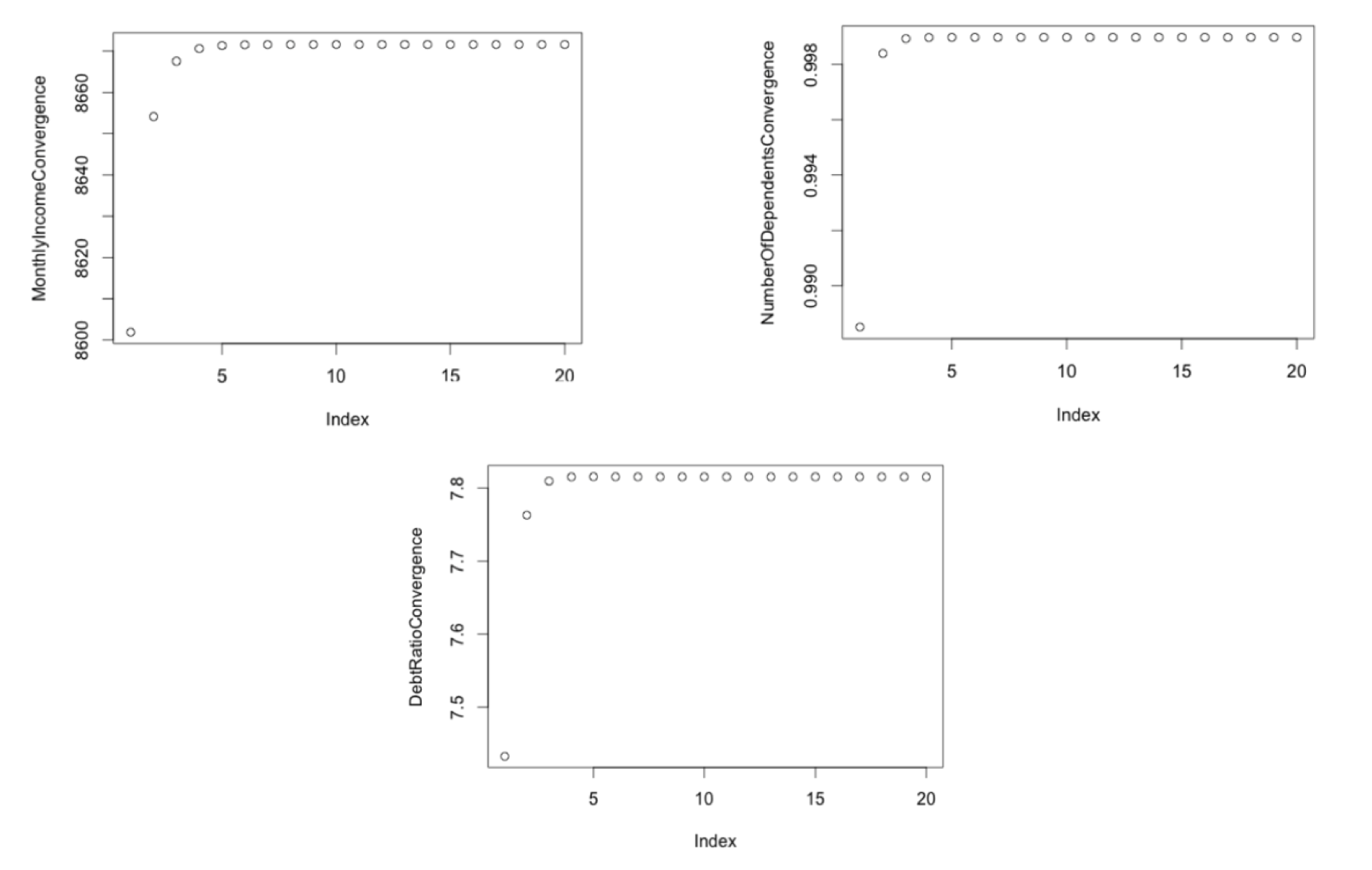
}Below we can see the values of each variable converging by looping through the linear models 20x as shown in the code above. The values actually converge more quickly than 20 iterations, in some cases only 3 iterations showed near convergence.
Train <- Impute(credit.train)
Train$SeriousDlqin2yrs <- SeriousDlqin2yrs
Test <- Impute(credit.pred)
Just to double check that the NA values do not exist anymore we can take a look at the NA sums over each variable and see they they have been replaced.
train_na2 <- as.data.frame(sapply(Train, function(x) sum(is.na(x))))
train_na2 <- data.frame(names = row.names(train_na2), count = train_na2[,1])

train_na2
## names count
## 1 RevolvingUtilizationOfUnsecuredLines 0
## 2 age 0
## 3 NumberOfTime30.59DaysPastDueNotWorse 0
## 4 DebtRatio 0
## 5 MonthlyIncome 0
## 6 NumberOfOpenCreditLinesAndLoans 0
## 7 NumberOfTimes90DaysLate 0
## 8 NumberRealEstateLoansOrLines 0
## 9 NumberOfTime60.89DaysPastDueNotWorse 0
## 10 NumberOfDependents 0
## 11 SeriousDlqin2yrs 0