
I wanted to annotate this out for everyone to read in case you wanted to take a look through it. This is an exploratory analysis of a completely random publicly available dataset found here from Piwowar HA, Vision TJ (2013). I had no prior knowledge of the data’s contents, but developed an understanding through some quick charts. Let’s take a look.
library(dplyr)
library(tidyr)
library(ggplot2)
library(knitr)
library(rgeos)
library(maps)
library(maptools)
library(gridExtra)
library(magrittr)
The first thing we want to know is how the data are delimited so we can decide how to read in the file for analysis. readLine() allows us to take a look at the rawdata which will give insight as to how the data are structured. All of those little \t’s that you see are the tabs. That’s how we know the data are tab delimited.
# Data are tab delimited
lines1 <- readLines("rawdata.txt", warn = FALSE)head(lines1)## [1] "pmid\tpubmed_issn\tpubmed_essn\tpubmed_year_published\tpubmed_date_in_pubmed\tpubmed_authors\tpubmed_journal\tpubmed_number_authors\tauthor_first_authors_first_name\tauthor_first_author_female\tauthor_first_author_male\tauthor_first_author_gender_not_found\tfirst_author_num_prev_pubs\tfirst_author_num_prev_pmc_cites\tfirst_author_year_first_pub\tfirst_author_num_prev_microarray_creations\tfirst_author_num_prev_oa\tfirst_author_num_prev_genbank_sharing\tfirst_author_num_prev_pdb_sharing\tfirst_author_num_prev_swissprot_sharing\tfirst_author_num_prev_geoae_sharing\tfirst_author_num_prev_geo_reuse\tfirst_author_num_prev_multi_center\tfirst_author_num_prev_meta_analysis\tauthor_last_author_first_name\tlast_first_author_female\tlast_first_author_male\tlast_first_author_gender_not_found\tlast_author_num_prev_pubs\tlast_author_num_prev_pmc_cites\tlast_author_year_first_pub\tlast_author_num_prev_microarray_creations\tlast_author_num_prev_oa\tlast_author_num_prev_genbank_sharing\tlast_author_num_prev_pdb_sharing\tlast_author_num_prev_swissprot_sharing\tlast_author_num_prev_geoae_sharing\tlast_author_num_prev_geo_reuse\tlast_author_num_prev_multi_center\tlast_author_num_prev_meta_analysis\taddress\tinstitution\tcountry\tgrant_numbers\tnum_grant_numbers\tnih_is_nci\tnih_is_nhlbi\tnih_is_ncrr\tnih_is_niehs\tnih_is_ninds\tnih_is_niddk\tnih_is_nigms\tnih_is_nichd\tnih_is_niaid\tpubmed_medline_status\tpubmed_is_review\tpubmed_is_humans\tpubmed_is_animals\tpubmed_is_mice\tpubmed_is_fungi\tpubmed_is_bacteria\tpubmed_is_plants\tpubmed_is_viruses\tpubmed_is_cultured_cells\tpubmed_is_cancer\tpubmed_is_open_access\tpubmed_is_effectiveness\tpubmed_is_diagnosis\tpubmed_is_prognosis\tpubmed_is_core_clinical_journal\tpubmed_is_clinical_trial\tpubmed_is_randomized_controlled_trial\tpubmed_is_meta_analysis\tpubmed_is_comparative_study\tpubmed_is_multicenter_study\tpubmed_is_validation_study\tpubmed_is_funded_stimulus\tpubmed_is_funded_nih_extramural\tpubmed_is_funded_nih_intramural\tpubmed_is_funded_non_us_govt\tpubmed_in_genbank\tpubmed_in_pdb\tpubmed_in_swissprot\tis_geo_reuse\tpubmed_number_times_cited_in_pmc\tfound_by_highwire\tfound_by_scirus\tfound_by_googlescholar\tportal_pmids_found_by_pmc\tpubmed_in_geo\tin_arrayexpress\tin_ae_or_geo\tcountry_clean\tinstitution_clean\tinstitution_hospital_or_medlcal\tinstitution_rank\tinstitution_sector\tinstitution_output\tinternational_collaboration\tinstitution_norm_sjr\tinstitution_norm_citation_score\tjournal_2008_cites\tjournal_impact_factor\tjournal_5yr_impact_factor\tjournal_immediacy_index\tjournal_num_articles_2008\tjournal_cited_halflife\tjournal_policy_tri\tjournal_policy_requires_microarray_accession\tjournal_policy_says_must_deposit\tjournal_policy_at_least_requests_sharing_microarray\tjournal_policy_mentions_any_sharing\tjournal_policy_general_statement\tjournal_policy_requests_accession\tjournal_policy_mentions_exceptions\tjournal_policy_mentions_consequences\tjournal_policy_contains_word_microarray\tjournal_policy_contains_word_MIAME_MGED\tjournal_policy_contains_word_arrayexpress\tjournal_policy_contains_word_geo_omnibus\tjournal_policy_requests_sharing_other_data\tpmid:1\tnum_grants\tlongest_num_years\tfirst_year\tlast_year\tcumulative_years\tsum_avg_dollars\tsum_sum_dollars\tmax_max_dollars\tnih_institutes\tgrant_activity_codes\thas_R01_funding\thas_T32_funding\thas_P01_funding\thas_R21_funding\thas_P30_funding\thas_P50_funding\thas_U01_funding\thas_R37_funding\thas_K_funding\thas_U_funding\tnum_post2004_morethan500k\tnum_post2003_morethan500k\tnum_post2005_morethan500k\tnum_post2006_morethan500k\tnum_post2007_morethan500k\tnum_post2003_morethan750k\tnum_post2004_morethan750k\tnum_post2005_morethan750k\tnum_post2006_morethan750k\tnum_post2007_morethan750k\tnum_post2003_morethan1000k\tnum_post2004_morethan1000k\tnum_post2005_morethan1000k\tnum_post2006_morethan1000k\tnum_post2007_morethan1000k"
## [2] "19450518\t0092-8674\t1097-4172\t2009\t38508.375\tMu??oz MJ;P??rez Santangelo MS;Paronetto MP;de la Mata M;Pelisch F;Boireau S;Glover-Cutter K;Ben-Dov C;Blaustein M;Lozano JJ;Bird G;Bentley D;Bertrand E;Kornblihtt AR\tCell\t14\tManuel\t0\t0\t0\t15\t146\t1995\t1\t0\t2\t0\t0\t0\t0\t0\t0\tAlberto\t0\t1\t0\t85\t1184\t1992\t1\t0\t10\t0\t0\t0\t0\t0\t0\t\"Laboratorio de Fisiolog??a y Biolog??a Molecular, Departamento de Fisiolog??a, Biolog??a Molecular y Celular, IFIBYNE-CONICET, Facultad de Ciencias Exactas y Naturales, Universidad de Buenos Aires, Ciudad Universitaria, Argentina.\"\tCiudad Universitaria\tArgentina\tGM58613\t1\t0\t0\t0\t0\t0\t0\t1\t0\t0\tindexed for MEDLINE\t0\t1\t0\t0\t0\t0\t0\t0\t1\t1\t0\t0\t1\t0\t0\t0\t0\t0\t0\t0\t0\t0\t1\t0\t1\t0\t0\t0\t0\t1\t0\t1\t1\t0\t0\t0\t0\tArgentina\tCiudad Universitaria\t0\t\t\t\t\t\t\t142064\t31.253\t30.149\t6.126\t348\t8.8\t2\t1\t1\t1\t1\t1\t2\t0\t0\t1\t1\t0\t0\t1\t19450518\t4\t6\t2003\t2008\t24\t2992315\t17953888\t416950\tGM\tR01\t1\t0\t0\t0\t0\t0\t0\t0\t0\t0\t0\t0\t0\t0\t0\t0\t0\t0\t0\t0\t0\t0\t0\t0\t0"
## [3] "16267287\t0021-9193\t1098-5530\t2005\t37237.375\tAlbanesi D;Mansilla MC;Schujman GE;de Mendoza D\tJ Bacteriol\t4\tDaniela\t1\t0\t0\t12\t60\t2000\t0\t0\t0\t0\t0\t0\t0\t0\t0\tDiego\t0\t1\t0\t63\t459\t1978\t1\t0\t10\t0\t0\t0\t0\t0\t0\t\"Instituto de Biolog??a Molecular y Celular de Rosario (IBR-CONICET) and Departamento de Microbiolog??a, Facultad de Ciencias Bioqu??micas y Farmac??uticas, Universidad Nacional de Rosario, Argentina.\"\tUniversidad Nacional de Rosario\tArgentina\t\t0\t0\t0\t0\t0\t0\t0\t0\t0\t0\tindexed for MEDLINE\t0\t0\t0\t0\t0\t1\t0\t0\t0\t0\t0\t0\t0\t0\t0\t0\t0\t0\t0\t0\t0\t0\t0\t0\t1\t0\t0\t0\t0\t3\t1\t0\t0\t0\t0\t0\t0\tArgentina\tUniversidad Nacional de Rosario\t0\t1314\tHigher educ.\t1234\t46.52\t1.03\t0.86\t58715\t3.636\t3.748\t0.892\t909\t9.6\t2\t1\t1\t1\t1\t0\t2\t0\t2\t1\t0\t1\t1\t1\t\t\t\t\t\t\t\t\t\t\t\t\t\t\t\t\t\t\t\t\t\t\t\t\t\t\t\t\t\t\t\t\t\t\t\t"
## [4] "17420266\t0022-1007\t1540-9538\t2007\t37786.375\tHorikawa K;Martin SW;Pogue SL;Silver K;Peng K;Takatsu K;Goodnow CC\tJ Exp Med\t7\tKeisuke\t0\t1\t0\t16\t56\t1984\t0\t0\t0\t0\t0\t0\t0\t0\t0\tChristopher\t0\t1\t0\t284\t4578\t1992\t1\t2\t4\t0\t0\t2\t0\t0\t0\t\"Immunogenomics Laboratory, The Australian Phenomics Facility, The John Curtin School of Medical Research, The Australian National University, Canberra 0200, Australia.\"\tThe Australian National University\tAustralia\t\t0\t0\t0\t0\t0\t0\t0\t0\t0\t0\tindexed for MEDLINE\t0\t0\t1\t1\t0\t0\t0\t0\t0\t0\t0\t0\t0\t0\t0\t0\t0\t0\t0\t0\t0\t0\t0\t0\t1\t0\t0\t0\t0\t5\t1\t0\t0\t0\t1\t1\t1\tAustralia\tAustralian National University\t1\t205\tHigher educ.\t9409\t49.98\t1.03\t1.42\t67322\t15.463\t15.504\t3.078\t245\t8.2\t2\t1\t1\t1\t1\t1\t2\t0\t2\t1\t1\t0\t0\t1\t\t\t\t\t\t\t\t\t\t\t\t\t\t\t\t\t\t\t\t\t\t\t\t\t\t\t\t\t\t\t\t\t\t\t\t"
## [5] "15802471\t0027-8424\t1091-6490\t2005\t37045.375\tSrikhanta YN;Maguire TL;Stacey KJ;Grimmond SM;Jennings MP\tProc Natl Acad Sci U S A\t5\tYogitha\t0\t0\t1\t7\t99\t1998\t0\t0\t3\t0\t0\t0\t0\t0\t0\tMichael\t0\t1\t0\t49\t564\t1992\t0\t0\t20\t0\t0\t0\t0\t0\t0\t\"School of Molecular and Microbial Science and Institute for Molecular Bioscience, University of Queensland, St. Lucia, Brisbane, Queensland 4072, Australia.\"\tUniversity of Queensland\tAustralia\t\t0\t0\t0\t0\t0\t0\t0\t0\t0\t0\tindexed for MEDLINE\t0\t0\t0\t0\t0\t1\t0\t0\t0\t0\t0\t0\t0\t0\t0\t0\t0\t0\t0\t0\t0\t0\t0\t0\t1\t0\t0\t0\t0\t10\t1\t0\t1\t1\t0\t0\t0\tAustralia\tUniversity of Queensland\t0\t\t\t\t\t\t\t416018\t9.38\t10.228\t1.635\t3508\t7.4\t2\t1\t1\t1\t1\t1\t2\t1\t0\t1\t1\t0\t1\t1\t\t\t\t\t\t\t\t\t\t\t\t\t\t\t\t\t\t\t\t\t\t\t\t\t\t\t\t\t\t\t\t\t\t\t\t"
## [6] "11526234\t0027-8424\t1091-6490\t2001\t35707.41736\tWatts RA;Hunt PW;Hvitved AN;Hargrove MS;Peacock WJ;Dennis ES\tProc Natl Acad Sci U S A\t6\tR\t0\t0\t1\t4\t74\t2001\t0\t0\t1\t0\t0\t0\t0\t0\t0\tE\t0\t0\t1\t82\t1303\t1978\t0\t0\t30\t1\t1\t0\t0\t0\t0\t\"CSIRO Plant Industry, Canberra, ACT 2601, Australia.\"\t\tAustralia\t\t0\t0\t0\t0\t0\t0\t0\t0\t0\t0\tindexed for MEDLINE\t0\t0\t1\t0\t0\t0\t1\t0\t0\t0\t0\t0\t0\t0\t0\t0\t0\t0\t1\t0\t0\t0\t0\t0\t0\t1\t0\t0\t0\t9\t1\t0\t1\t0\t0\t0\t0\tAustralia\t\t0\t\t\t\t\t\t\t416018\t9.38\t10.228\t1.635\t3508\t7.4\t2\t1\t1\t1\t1\t1\t2\t1\t0\t1\t1\t0\t1\t1\t\t\t\t\t\t\t\t\t\t\t\t\t\t\t\t\t\t\t\t\t\t\t\t\t\t\t\t\t\t\t\t\t\t\t\t"So to read in this file we will use data.table with sep = "\t". This tells R that instead of a typical excel file that is delimited with commas (.csv), we are now delimited with tabs. Some of you may notice the occasional ?? occurring in the data. This is actually in the original dataset and not a product of reading error through R. Future analysis could attempt to remove these inconsistencies before any learning algorithm is implemented. fill = TRUE is necessary here because the data have portions of unequal rows, so read.table fills the remainder of the row to keep constant dimension.
rawdata <- read.table("rawdata.txt", header = TRUE, sep = "\t",
                      fill = TRUE, quote = "", comment.char = "",row.names = NULL,
stringsAsFactors = FALSE)dim(rawdata)## [1] 11603 158Now we use our trusty str() to take a much closer look at the structured dataset.
# Observe all variables
str(rawdata, list.len=ncol(rawdata))
One good thing to do before looking at multicollinearity or varaible relationships is to break up the data into numerical and character. rawdata[, sapply(rawdata, is.numeric)] takes the dataset and runs over the columns asking if each value is numeric, if it is then we subset those columns of rawdata and assign them to a new object called data_numr.
I also took all of the blank spaces in the character matrix and gave them a value of NA.
# Break up character and numerical
data_numr = rawdata[, sapply(rawdata, is.numeric)]
data_char = rawdata[, sapply(rawdata, is.character)]
data_char[data_char==""] = NA
Now we try to get a sense of how many NA values we are working with. sapply(data\_numr, function(x) sum(is.na(x))) will run through and ask if each value is an NA, and if it is is.na() will give a TRUE, and summing all of those TRUEs gives the number of NA values. Then we just row bind the data into one big data frame and only take the non-zero ones. Setting breaks <- c(50,100,250,500,1000,2000,5000,10000) allows us to define the breaks in the histogram directly later on. If you run table(all\_na) you will see where aes(x = count, fill=type) comes from.
num_na = sapply(data_numr, function(x) sum(is.na(x)))
char_na = sapply(data_char, function(x) sum(is.na(x)))
all_na = rbind(data.frame(count=num_na, type="Numerical"),
               data.frame(count=char_na, type="Character"))
# table(all_na)
all_na = data.frame(all_na)
all_na = all_na[all_na$count>0,]

breaks <- c(50,100,250,500,1000,2000,5000,10000)

ggplot(all_na, aes(x = count, fill=type)) +
  geom_histogram(alpha=0.7) +
  scale_x_log10(limits=c(50,12000), breaks=breaks) +
  labs(title="Histogram of Feature Count per NA Count", size=24, face="bold") +
  xlab("NA Count") + ylab("Feature Count")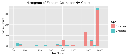
We can see there are various amounts of missing data throughout the features, so I will take a closer look at a few of them. This is just percent calculation dividing the missing data and the number of rows. !is.na() does the opposite of is.na(), it gives TRUEs for all of the non-NA values. cat() will perform whatever function or operation we are asking, and then follow up the result with some text. So in this case I used it to just calculate the percentage and then followed it by "% data available".
cat((sum(!is.na(rawdata$sum_avg_dollars))/dim(rawdata)[1])*100, "% data available")## 26.40696 % data available# journal_immediacy_index - the average number of times an article is cited in the year it is published
cat((sum(!is.na(rawdata$journal_immediacy_index))/dim(rawdata)[1])*100, "% data available")## 91.37292 % data availablecat((sum(!is.na(rawdata$found_by_googlescholar))/dim(rawdata)[1])*100, "% data available")## 100 % data availableFrom looking at our data earlier, we saw that two variables had country names in them. Upon closer inspection, one of them is called country_clean which is a cleaned up version of the original country column. This is great for us because it saves us work in cleaning the country names. So we want to see the distribution of these names in a heat map across the world map. For this we will begin with the map() function, or as I like to call it, Dora’s function.
The map() function has a number of databases, one of which is entitled world, which gives us a clear look at the world map, delineated by countries. If we take a look within our mapWORLD there’s a variable called $names. Some of the elements in $names contain a :. We will break each of these character strings at the colon and only select the first character string after the split for our new variable nms. (e.g. if I have Sweden:Oland, strsplit() will break the string into two strings by splitting it at the : and dividing it in two. Then we only select the first element of this division, which is the piece we actually want).
Now we need to convert things from ‘Dora’s function’ map() to something that our sp package can use. That’s where map2SpatialPolygons() comes in. (This code is straight out of “Applied Spatial Data
Analysis with R” Bivand et al, in case you are interested) We pass this function our map() output, our IDs, and then specify the proj4string argument as CRS('+proj=longlat'). CRS stands for ‘coordinate reference system’ and +proj=longlat is accepted for geographical coordinates, which essentially means we have a vector of a bunch of latitudes and longitudes. We will see soon why we needed to create this variable.
Now we make the function that actually draws the heat map on the world map. mapCountries accepts a data frame and a feature from that dataframe to construct the heat map. We already know what we want to pass this function (our data frame of character features and the variable with country names). dat becomes our data frame, which we create from the column in df that is the feature passed into the function. The interesting part to this line of code is the use of table(). table() orders all of the factor levels and then gives the count that they occur. names() gives us the character strings of our variable names, if we pass the names of our data frame the two values country (string of 50 state abbreviations) and value, we are forcing the variable names to be these values and therefore we have an ordered set of country names and then value as the number of occurences.
Now we create a vector of the positions where country names in dat$country and in nms align, this is saved as idx. We now create a data frame dat2 that contains all of the unique country names that occur in nms and then the number of times that name occurs in the entire variable column from our train_char. All data frames have row names, but they kind of go unnoticed. Here we utilize them and give them the names of the countries that occur in nms. Now we have perfect country names and counts.
Remember a long time ago when we made the WORLDpolygons object that included that mess created by map2SpatialPolygons()? Well now we get to use that mess with the SpatialPolygonsDataFrame() function. This is the final formatting needed to pass through spatial data for plotting. Finally, our function will use the spplot() function from the sp package to plot the heat maps. Then we just call this function on our train_char and the two features of interest.
mapWORLD <- map('world', fill=TRUE, plot=FALSE)
nms <- sapply(strsplit(mapWORLD$names,  ':'),  function(x)x[1])
WORLDpolygons <- map2SpatialPolygons(mapWORLD,  IDs = nms,  CRS('+proj=longlat'))

mapCountries = function(df, feat){
  dat = data.frame(table(df[,feat]))
  names(dat) = c("country", "value")

  idx <- match(unique(nms),  dat$country)
  dat2 <- data.frame(value = dat$value[idx], country = unique(nms))
  row.names(dat2) <- unique(nms)
  WORLDsp <- SpatialPolygonsDataFrame(WORLDpolygons,  data = dat2)
  spplot(WORLDsp['value'], main=paste(feat, "frequency"), col.regions=rev(heat.colors(21)))
}
mapCountries(data_char, "country_clean")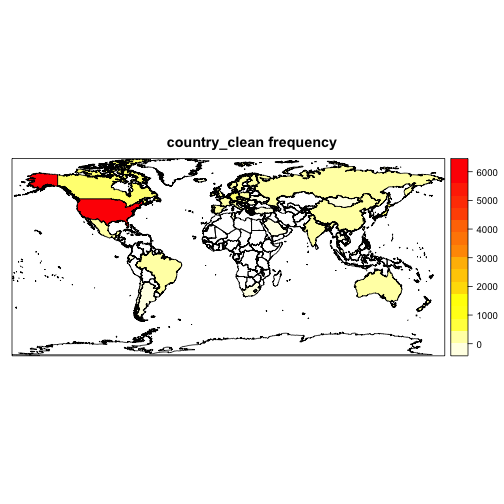
Here I wanted to take a look at the authors’ previous publications count. I thought this could be interesting if we could later relate this back to how much funding their project received. mutate() creates a new variable in our dataframe, and here I defined it to be the sum of the first author’s prev_pubs and the last author’s.
rawdata <- rawdata %>% mutate(prev_pubs = first_author_num_prev_pubs + last_author_num_prev_pubs)
pub_count <- data.frame(rawdata$prev_pubs, rawdata$found_by_googlescholar)
pub_count$rawdata.found_by_googlescholar <- as.factor(pub_count$rawdata.found_by_googlescholar)
Now I just create a histogram in ggplot() using the value calculated with the pub_count. There’s a fairly large range in the distribution of authors’ previous publication count.
ggplot(pub_count, aes(x = rawdata.prev_pubs, fill = rawdata.found_by_googlescholar)) +
  geom_histogram() +
  stat_bin(binwidth = 100) +
  scale_fill_discrete(name = "Shown in\nGoogle Scholar\nSearch") +
  labs(title="Histogram of Authors' Previous Publications", size=24, face="bold") +
  xlab("Number of Publications for First and Last Author") + ylab("Frequency")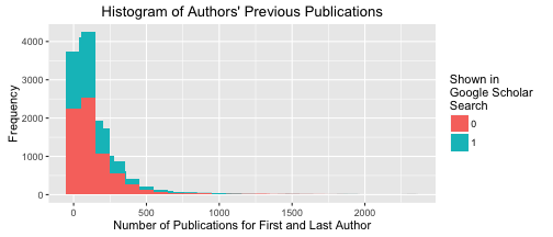
Here I wanted to take a look at the funding, naturally we must follow the money. Specifically I wanted to create a histogram that showed how much funding each project was receiving while breaking each project up according to the type of funding they were receiving.
If you know that you want to select() multiple columns in a row, we may use a : to indicate the first column through the last column, i.e. has _R01_funding:has_U_funding. You use mutate_each_ with the extra underscore if you want to supply what I wrote as cols as a string/variable. factor(.) forces all of the columns to be factor variables. Typically in R we indicate all columns in a matrix with .
data_fund <- rawdata %>% select(sum_avg_dollars, has_R01_funding:has_U_funding)
cols <- c("has_R01_funding", "has_T32_funding", "has_P01_funding",
          "has_R21_funding", "has_P30_funding", "has_P50_funding",
          "has_U01_funding", "has_R37_funding", "has_K_funding",
          "has_U_funding")
data_fund <- data_fund %>% mutate_each_(funs(factor(.)),cols)
str(data_fund)
## 'data.frame': 11603 obs. of 11 variables:
## $ sum_avg_dollars: int 2992315 NA NA NA NA NA NA NA NA NA ...
## $ has_R01_funding: Factor w/ 2 levels "0","1": 2 NA NA NA NA NA NA NA NA NA ...
## $ has_T32_funding: Factor w/ 2 levels "0","1": 1 NA NA NA NA NA NA NA NA NA ...
## $ has_P01_funding: Factor w/ 2 levels "0","1": 1 NA NA NA NA NA NA NA NA NA ...
## $ has_R21_funding: Factor w/ 2 levels "0","1": 1 NA NA NA NA NA NA NA NA NA ...
## $ has_P30_funding: Factor w/ 2 levels "0","1": 1 NA NA NA NA NA NA NA NA NA ...
## $ has_P50_funding: Factor w/ 2 levels "0","1": 1 NA NA NA NA NA NA NA NA NA ...
## $ has_U01_funding: Factor w/ 2 levels "0","1": 1 NA NA NA NA NA NA NA NA NA ...
## $ has_R37_funding: Factor w/ 2 levels "0","1": 1 NA NA NA NA NA NA NA NA NA ...
## $ has_K_funding : Factor w/ 1 level "0": 1 NA NA NA NA NA NA NA NA NA ...
## $ has_U_funding : Factor w/ 1 level "0": 1 NA NA NA NA NA NA NA NA NA ...Each funding variable is a 1 if it is that type of funding or a 0 if it’s not. So What we want is one column that has a factor level for each of the types of funding, arranged by the dollars funded. data_fund %>% gather(funding, yes, -sum_avg_dollars) we pipe in data_fund dataframe using our piping operator %>%, and then we use gather() which puts all of the columns selected into rows with new variables funding (the key) and yes which is whether or not the study had that funding type. Then we filter() for only the rows with a yes value of 1, which means they had that funding type and then arrange() each by the amount of funding.
data_fund <- data_fund %>% gather(funding, yes, -sum_avg_dollars) %>%
  filter(yes == 1) %>% select(-yes) %>% arrange(sum_avg_dollars)
data_fund$funding <- as.factor(data_fund$funding)
Now we plot this with a ggplot() histogram.
ggplot(data_fund, aes(x = sum_avg_dollars, fill=funding)) +
  geom_histogram(alpha=0.7) +
  scale_x_log10(limits=c(100000,1500000000)) +
  labs(title="Histogram of Funding Arranged by Type", size=24, face="bold") +
  xlab("Funding") + ylab("Frequency")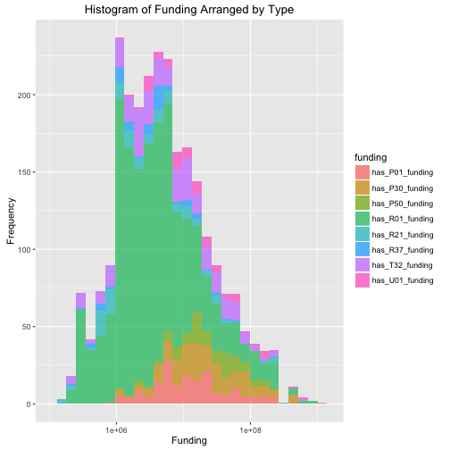
Outside googling led me to find that the reward names refer to: Program and Cooperative Awards (P01, P20, P50, U01), Individual Research Awards (R01, R21, and R37), and Institutional Award (T32).
Now that I have procrastinated my actual homework enough I think it’s time to get back to it. Feel free to add some analysis and send it to me. I’m always intrigued.