
The goal here is to naively run through the entire support of permuting the integers of length $m$ and then determining the ones that are “big” permutations, i.e. $\Sigma i x_i > k$.
So more formally, suppose we want a random permutation $x = (x_1, x_2, … , x_m)$ of the integers $1, … , m$ that satisfies $\Sigma i x_i > k$. For a given value of $m$, there are $n(k)$ of these, so each should have probability $\frac{1}{n(k)}$. However, finding these permutation is computationally infeasible for moderate $m$ (as it requires checking $m!$ permutations).
Suppose we are at state $x$ (a particular permutation). Define a neighbor of $x$ as a permutation satisfying the constraint that is achieved by switching two elements of $x$. Suppose $x$ has $N(x)$ neighbors. Let $y$ be one of those neighbors, and $y$ has $N(y)$ neighbors. These quantities are easy to calculate as it only requires checking $\choose{m,2}$ permutations, much smaller than $m!$. At each iteration, randomly select a neighbor and move to it with probability $min(1, \frac{N(x)}{N(y)})$. Then the stationary distribution is the one we wanted. $p_{xy}$ is the probability that we are at $x$ and move to $y$. Suppose $N(y)$ is less than $N(x)$. First we need to be offered a move to $y$, with probability $\frac{1}{N(x)}$. Then, because $N(y)$ is less than $N(x)$, we necessarily move to it. So $p_{xy} = \frac{1}{N(x)}$. $p_{xy}$ is the chance that we move from $y$ to $x$, so first we must be offered $x$, with probability $\frac{1}{N(y)}$, then we must decide to move there, with probability $\frac{N(y)}{N(x)})$ so $p_{yx} = \frac{1}{N(x)}$ as well. Since the transition probabilities are the same, the stationary probabilities for $x$ and $y$ must also be the same (from the above).
This code runs through every permutation and gives the size $k$ of the permutations that are one two-swap away from each other. Then the average of the permuations gives the stationary distribution. We can see in the graphs below that the line graph converges on the stationary distribution and the histogram represents the frequency of permutation sizes.
So we can see an algorithm emerge here where
- Given $x^t$
- Generate $Y_t \sim g(y - x^t)$
- Take \(X^{t+1} = \begin{cases} Y_t \text{ with probability } \text{min}\{1, \frac{f(Y_t)}{f(x^t)}\} \\ x^t \text{ otherwise} \end{cases}\)
To get a better sense of this problem, let us look at a deck of cards that need to be shuffled. The rules of the shuffle are that at each time step, choose two positions $i$ and $j$ randomly in the deck. Take the cards at those positions, and swap them. If the Markov chain $P$ is defined by these transitions, is $P$ irreducible? Yes: it is not hard to show that with a sequence of $n$ pair swaps, we can generate any permutation we want. Is $P$ aperiodic? Yes: if we allow the possibility of $i$ and $j$ being the same card we have self-loops. So $P$ is ergodic and converges to its stationary distribution. This Markov chain is reversible, and moreover $P$ is entirely symmetric so $\pi_x = \pi_y$. This tells us that after running long enough, this random transposition will sample each permutation of the deck of cards with equal probability.
Our goal here is to essentially explore the entire support of the density according to its probability. Because of its symmetric features, it spends about half the time of the simulation running over areas of the support it has already been to. Our method is very similar to Accept-Reject method in the sense that the instrumental distribution is the same density $g$ as in rejection method. We can see on the line plots of sizes according to their index that for some intervals of time the sequence does not change at all because the cooresponding $Y_i$’s are being rejected. This is one area where we can see a difference between this method and Accept-Reject method. This sampling will have repeated occurences of the same value since rejection of $Y$ brings about repetition of $X^{t}$ at time $t+1$.
One can imagine that when the acceptance system is offered an area of the support that it hasn’t been to in a while, it wants to go there. However, keep in mind that the acceptance probability does not depend on the symmetric proposal density $g$. Changing $g$ will give different values of $Y_t$’s but the dependence does not exist. But there does exist a dependence between the candidate distribution and the current state of the chain. Actually, a high acceptance rate does not indicate the method is doing what we want it to. The algorithm may just be moving to slowly across the support. If the acceptance rate is low, the algorithm may be moving more quickly over the support and reaches the “borders”, exploring regions with low probability under $f$.
Size <- function(List){
  # Calculates "Size" of Permutation
  #
  # Args:
  #   List: Permutation whose size is to be calculated
  #
  # Returns:
  #   Size of Vector
  M <- length(List)
  return(sum(List * seq(1:M)))
}
Neighbors <- function(List,k){
# Finds 2 swap neighbors of a given Permutation still larger than k
#
# Args:
# List: Permuation whose neighbors we want
# k: size of a permutation required to be "big"
#
# Returns:
# Returns list with number of neighbors and all the neighbors
M <- length(List)
max_nNeighbors <- factorial(M) / (factorial(2) * factorial(M-2)) #M choose 2
List_Neighbors <- vector("list",round(max_nNeighbors)) # initializes list of Neighbors
nNeighbors <- 0 # initializes count of number of neighbors
l <- 1 # initializes index for list of neighbors
#walks through all 2 swap permutations (neighbors)
for (i in 1:(M-1)) {
for(j in (i+1):M) {
swap2 <- List
swap2[i] <- List[j]
swap2[j] <- List[i]
size <- Size(swap2)
if (size > k){ # if neighbor is big
List_Neighbors[[l]] <- swap2 # store neighbor
nNeighbors <- nNeighbors + 1 # increments number of neighbors
l <- l + 1
}
}
}
return(c(nNeighbors,List_Neighbors))
}BigListAvg <- function(M,k) {
# Calculates average size of Permutations with size > k
#
# Args:
# M: Length of sequence
# k: size of a permutation required to be "big"
#
# Returns:
# Average size of big Permutations
max_list <- c(seq(1:M)) # Largest Permutation
max_size <- Size(max_list) # Largest Size
if (k > max_size){
stop(paste('k larger than maximum size: ', max_size, sep=''))
}
X <- max_list # initializes X at largest permutation
tempX <- Neighbors(X,k)
nX <- tempX[[1]] # number of neighbors for X
neighbors <- tempX[2:(nX + 1)] # all the neighbors of X
sizes <- c() # initializes vector of sizes
j <- 0 # initializes index for vector of sizes
for (i in 1:100){
Y <- neighbors[[runif(1,1,nX + 1)]] # randomly chooses neighbor of X
tempY <- Neighbors(Y,k)
nY <- tempY[[1]] # number of neighbors for X
p <- min(1, nX/nY) # probability of moving from X to Y
U <- runif(1,0,1)
if (U < p) {
X <- Y
nX <- nY
neighbors <- tempY[2:(nY + 1)]
}
j <- j + 1
sizes[j] <- Size(X) # records size of current permutation
}
par(mfrow=c(1,2))
plot(sizes[20:j],type="l", main = paste("M = ", M, "and k =", k)) # remove first 20 iterations to unbias stationary dist
hist(sizes, breaks = 30)
avg_size <- mean(sizes) # calculates mean size of all big permutations walked through
cat("The average size is",avg_size)
}BigListAvg(10,350)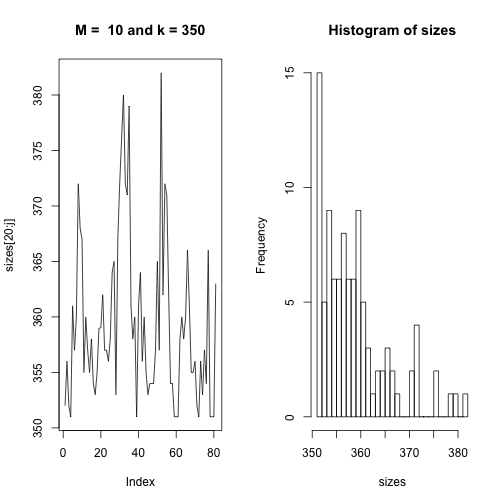
## The average size is 359.21BigListAvg(50,42000)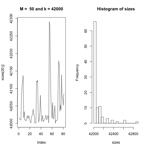
## The average size is 42079.5BigListAvg(100,330000)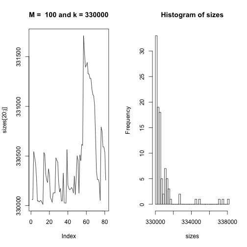
## The average size is 330806.4