Let’s take a look at a Kaggle competition dataset and R code from author, Darragh. One of the interesting things about this Kaggle dataset is that we don’t know much about the set itself and we need to figure everything out from scratch. That is what this code does well and we will break down each piece of it to make sure we understand how and why it is done. Remember, each time we encounter a new chunk of code we should be thinking why is this necessary, or, what is it we want to do next? I’ve included little statements about our ‘Goals’ to get you started thinking this way. Here is the website of the Kaggle competition, and you can obtain this code through the generosity of Darragh.
Goal: to explore the dataset and get a better sense of the variables.
So let’s get started.
“Sys.time()” is taking the current time when you ran the code at your system’s location. We save that to some variable “time.1” and then we use the “format()” function to display the time nicely. The second argument is a character string that pulls each part of the time (day, month, year – hour, minute, second).
time.1 <- Sys.time()
format(time.1, "%d-%m-%Y--%H:%M:%S")
## [1] "25-03-2016--19:12:58"All of the “library()” commands allow us to utilize these packages later on in the analysis. We need to remember though that this cannot be run unless we first install.packages(“”) for each of these packages. This can also be done by clicking on “tools” in the menu bar and then “Install Packages…”. There is a function “set.seed()” that is a way to control our randomness. If we choose to use this function, for any function we use later on that uses some kind of random generation, we can now replicate that same result by using the same set.seed() value. If you are reproducing this code, try set.seed(294).
Some of you may notice that the “read_csv()” function has an underscore instead of a dot “read.csv()”. This is simply because we are using the read csv function from the “readr” package. The added benefit here is that we can delineate how many rows we want to read in the file in the second argument (set to 20000). This is beneficial since the dataset is so large and we really just want to get a sense of what it looks like and different relationships between features.
We also redefine train to be a ‘subset’ of itself. We pass the function subset ‘train’, which is our dataset to train our model on (only the first 20,000 rows) and tell it to select all columns except for ‘ID’ and ‘target’. This last step is achieved using the select argument in the subset function and using a negative sign before concatenating the columns i.e. select=-c(ID, target).
We then get the total row count of our “train.csv” file, which tells us there are 145232 rows, and save this number into a variable called ‘row_count’. Finally, the cat() function is very similar to the c() -> concatenate function, however, cat() will also print the result. We can manipulate the output by passing text strings followed by the varaible we want to print so that it prints nice and tidy. Here we print the string “Row count : “ followed by the ‘row_count[1]’, which just means the first element of the variable row_count. We then print the string “Predictor column count : “ followed by the ‘ncol(train)’, which calculates the number of columns in our train dataset.
train <- read_csv("train.csv", n_max=20000)y = train$target
# remove the id and target
train = subset(train, select=-c(ID, target))
# get the rowcount
row_count = countLines("train.csv")
cat("Row count : ", row_count[1], "; Predictor column count : ", ncol(train))## Row count : 145232 ; Predictor column count : 1932Goal: to find the features that will actually help our model later on.
‘is.na’ is a fantastic function which returns a logical vector of the same length indicating whether a value is missing or not (TRUE means the element is missing). For this function we are essentially saying, take all of the missing elements of train, then take the length of that vector, and divide it by the total dimensions of the dataset ‘train’. Remember that whenever we use the brackets next to an object, we are essentially saying ‘the elements of’ that object. Then the number of columns times the number of rows is just the dimension of the matrix.
length(train[is.na(train)])/(ncol(train)*nrow(train))## [1] 0.005719203Sometimes a dataset can contain duplicate rows, this is good data cleaning practice to check for duplicates. For this we use the unique() function, which simply returns the same thing that you passed it, but with duplicates removed. and just subtract the number of rows from total rows. This value should be zero. And it is!
nrow(train) - nrow(unique(train))## [1] 0Sometimes columns can contain all the same value for each row. This isn’t very useful to us so we will just remove these columns. But first, we need to locate them.
‘col_ct’ will pass over the features of our ‘train’ dataset return the number of unique elements in the column. This is the great effect of the sapply() function. We can pass our function that we defined on the fly, i.e. length(unique(x), and apply it to all the elements of ‘train’. Now we want to know how many of them returned a value of 1. Because these are the features that all have the same value, or are considered constant features. We can then redefine train as only those columns that are not the ones that are constant features. Recall that when we use brackets on a matrix or array, we can delineate just the columns by placing a comma directly after the open bracket i.e. train[, …]. An exclamation point prior to an object is saying ‘not these elements’. And piping multiple functions together is done using commands such as, %.% or %>% or %in% (used in our case). So in our own words, we can read this line as, assign ‘train’ as only those columns in train that are not the names in those of the constant features.
col_ct = sapply(train, function(x) length(unique(x)))
cat("Constant feature count:", length(col_ct[col_ct==1]))
## Constant feature count: 5# we can just remove these columns
train = train[, !names(train) %in% names(col_ct[col_ct==1])]Goal: separate the numeric and non-numeric rows.
To get a sense of all of our feature vectors, we must deal with them as numeric and character vectors. To do this we will separate the dataset into sections (numeric and character). Again we are using many of the same functions we discussed earlier. ‘is.numeric()’ and ‘is.character’ are much like ‘is.na()’, except instead of returning trues and falses where there are NA values, they perform this for whether values are numeric or character strings.
The function ‘dim()’ returns the dimensions of a matrix/array/data frame, which is the rows by columns. Since we want to know how many variables we are dealing with, we only want the number of columns. So we take the second element of what dim(train_numr) returns and print it as the number of numeric columns. Then we do the same for character featrues. There are way more numerical features than character ones.
train_numr = train[, sapply(train, is.numeric)]
train_char = train[, sapply(train, is.character)]
cat("Numerical column count : ", dim(train_numr)[2],
    "; Character column count : ", dim(train_char)[2])
## Numerical column count : 1876 ; Character column count : 51Goal: learn more about character features.
Since we know there are only 51 character features, we can actually take a look at all of them without our brains exploding. We apply the function ‘unique()’ to all of the character features, and then we print the first 4 of them (if there are 4).
str(lapply(train_char, unique), vec.len = 4)## List of 51
## $ VAR_0001: chr [1:3] "H" "R" "Q"
## $ VAR_0005: chr [1:4] "C" "B" "N" "S"
## $ VAR_0008: chr [1:2] "false" ""
## $ VAR_0009: chr [1:2] "false" ""
## $ VAR_0010: chr [1:2] "false" ""
## $ VAR_0011: chr [1:2] "false" ""
## $ VAR_0012: chr [1:2] "false" ""
## $ VAR_0043: chr [1:2] "false" ""
## $ VAR_0044: chr [1:2] "[]" ""
## $ VAR_0073: chr [1:1094] "" "04SEP12:00:00:00" "26JAN12:00:00:00" "18SEP12:00:00:00" ...
## $ VAR_0075: chr [1:1776] "08NOV11:00:00:00" "10NOV11:00:00:00" "13DEC11:00:00:00" "23SEP10:00:00:00" ...
## $ VAR_0156: chr [1:399] "" "14JUL11:00:00:00" "21NOV11:00:00:00" "13APR12:00:00:00" ...
## $ VAR_0157: chr [1:120] "" "05JUL12:00:00:00" "05JUN11:00:00:00" "26MAY12:00:00:00" ...
## $ VAR_0158: chr [1:161] "" "31JAN12:00:00:00" "01MAR12:00:00:00" "02JAN12:00:00:00" ...
## $ VAR_0159: chr [1:374] "" "14JUL11:00:00:00" "21NOV11:00:00:00" "13APR12:00:00:00" ...
## $ VAR_0166: chr [1:1069] "" "12MAR12:00:00:00" "25FEB12:00:00:00" "22DEC11:00:00:00" ...
## $ VAR_0167: chr [1:260] "" "09JUN12:00:00:00" "21MAY12:00:00:00" "07AUG10:00:00:00" ...
## $ VAR_0168: chr [1:753] "" "22MAR12:00:00:00" "26JAN12:00:00:00" "22AUG11:00:00:00" ...
## $ VAR_0169: chr [1:940] "" "12MAR12:00:00:00" "25FEB12:00:00:00" "13JAN12:00:00:00" ...
## $ VAR_0176: chr [1:1133] "" "12MAR12:00:00:00" "25FEB12:00:00:00" "14JUL11:00:00:00" ...
## $ VAR_0177: chr [1:330] "" "09JUN12:00:00:00" "05JUL12:00:00:00" "21MAY12:00:00:00" ...
## $ VAR_0178: chr [1:758] "" "22MAR12:00:00:00" "26JAN12:00:00:00" "22AUG11:00:00:00" ...
## $ VAR_0179: chr [1:939] "" "12MAR12:00:00:00" "25FEB12:00:00:00" "14JUL11:00:00:00" ...
## $ VAR_0196: chr [1:2] "false" ""
## $ VAR_0200: chr [1:5031] "FT LAUDERDALE" "SANTEE" "REEDSVILLE" "LIBERTY" ...
## $ VAR_0202: chr [1:2] "BatchInquiry" ""
## $ VAR_0204: chr [1:1191] "29JAN14:21:16:00" "01FEB14:00:11:00" "30JAN14:15:11:00" "01FEB14:00:07:00" ...
## $ VAR_0214: chr [1:2] "" "HRE-Home Phone-0621"
## $ VAR_0216: chr [1:2] "DS" ""
## $ VAR_0217: chr [1:398] "08NOV11:02:00:00" "02OCT12:02:00:00" "13DEC11:02:00:00" "01NOV12:02:00:00" ...
## $ VAR_0222: chr [1:2] "C6" ""
## $ VAR_0226: chr [1:3] "false" "true" ""
## $ VAR_0229: chr [1:2] "false" ""
## $ VAR_0230: chr [1:3] "false" "true" ""
## $ VAR_0232: chr [1:3] "true" "false" ""
## $ VAR_0236: chr [1:3] "true" "false" ""
## $ VAR_0237: chr [1:44] "FL" "CA" "WV" "TX" ...
## $ VAR_0239: chr [1:2] "false" ""
## $ VAR_0274: chr [1:57] "FL" "MI" "WV" "TX" ...
## $ VAR_0283: chr [1:8] "S" "H" "-1" "P" ...
## $ VAR_0305: chr [1:8] "S" "P" "H" "-1" ...
## $ VAR_0325: chr [1:10] "-1" "H" "R" "S" ...
## $ VAR_0342: chr [1:49] "CF" "EC" "UU" "-1" ...
## $ VAR_0352: chr [1:5] "O" "R" "U" "-1" ...
## $ VAR_0353: chr [1:5] "U" "R" "O" "-1" ...
## $ VAR_0354: chr [1:5] "O" "R" "-1" "U" ...
## $ VAR_0404: chr [1:393] "CHIEF EXECUTIVE OFFICER" "-1" "CONTA" "CONTACT" ...
## $ VAR_0466: chr [1:3] "-1" "I" ""
## $ VAR_0467: chr [1:5] "-1" "Discharged" "Dismissed" "" ...
## $ VAR_0493: chr [1:247] "COMMUNITY ASSOCIATION MANAGER" "-1" "LICENSED PRACTICAL NURSE" "LICENSED VOCATIONAL NURSE" ...
## $ VAR_1934: chr [1:5] "IAPS" "RCC" "BRANCH" "MOBILE" ...Goal: encode all NA values the same way.
“It looks like NA is represented in character columns by -1 or [] or blank values, lets convert these to explicit NAs.” We see here that our data is a little messy. The missing values are not already coded as NAs, so we must do this ourselves. Darragh remarks, “Not entirely sure this is the right thing to do as there are real NA values, as well as -1 values already existing, however it can be tested in predictive performance.” This is an issue with data cleaning that we may not be able to avoid.
train_char[train_char==-1] = NA
train_char[train_char==""] = NA
train_char[train_char=="[]"] = NA
Goal: put date features in new data frame.
Now we want to create a new dataframe for the date features. To do this we will use ‘grep()’. grep() will search through a character vector looking for the pattern that you tell it to look for. In this case our pattern that we pass it is JAN1 FEB1 MAR1. The same thing gets returned if you only pass the pattern “JAN1”.
train_date = train_char[,grep("JAN1|FEB1|MAR1", train_char),]Goal: remove dates from character features and view them separately.
“colnames(train_char) %in% colnames(train_date)” will give TRUE or FALSE where the column name in train_char is overlapped with that in train_date. Once we place the exclamation point in front, this just reverses all of the TRUEs and FALSEs (TRUE becomes FALSE, and vice versa). Then we want only those columns in train_char and we will redefine train_char in this way.
Now we will redefine train_date. ‘strptime()’ allows you to pass it the format that the date string is given in the variables, and it will convert it to the appropriate formatting for date and time. “%d%B%y” is “day, full month name, year (without century)”. Then we make a data frame by column binding the train_date vectors. Now we have dates and characters separate.
train_char = train_char[, !colnames(train_char) %in% colnames(train_date)]
train_date = sapply(train_date, function(x) strptime(x, "%d%B%y:%H:%M:%S"))
train_date = do.call(cbind.data.frame, train_date)
Goal: separate times from dates.
Now we can separate the dates and the times. Just from looking at our data frame, we can see that only variables VAR_0204 and VAR_0217 contain times.
‘train_hour’ utilizes the ‘substr()’ function to grab only the first two digits of the time (aka the hour).
train_time = train_date[,colnames(train_date) %in% c("VAR_0204","VAR_0217")]
train_time = data.frame(sapply(train_time, function(x) strftime(x, "%H:%M:%S")))
train_hour = as.data.frame(sapply(train_time, function(x) as.numeric(as.character(substr( x ,1, 2)))))
Now we want to plot a histogram of the dates. If we take a look at “dim(train_date)”, we can see that there are 16 columns. The “weeks” argument is defined as the breaks in the histogram. This is the name of an algorithm that R reads a sets the breakpoints to nice values for our data. Lower case %b is the abbreviated month name.
par(mar=c(2,2,2,2),mfrow=c(4,4))
for(i in 1:16) hist(train_date[,i], "weeks", format = "%d %b %y", main = colnames(train_date)[i], xlab="", ylab="")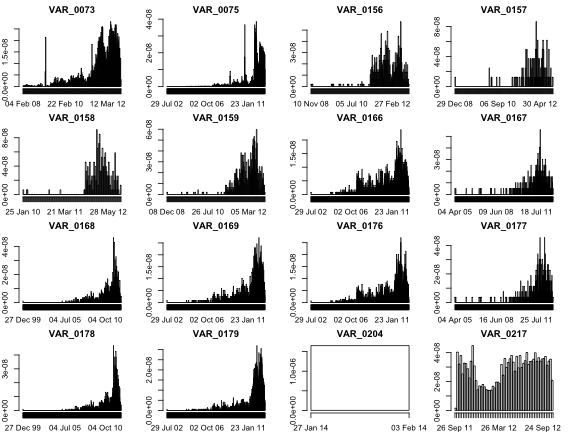
Now if we want histograms of the times, the process is pretty much the same. Nothing new to see here in the code.
par(mar=c(2,2,2,2),mfrow=c(1,2))
for(i in 1:2) hist(train_hour[,i], main = paste(colnames(train_hour)[i], "hourly"), breaks = c(0:24), xlab="", ylab="")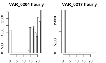
Goal: view geographical elements of variables containing state names.
From looking at our data earlier, we saw that two variables had abbreviations of states as their elements. So we want to see the distribution of these abbreviations in each variable in a heat map across the US map. For this we will begin with the ‘map()’ function, or as I like to call it, Dora’s function.
The map() function has a number of databases, one of which is entitled ‘state’, which gives us a clear look at the US map, delineated by states. If we take a look within our ‘mapUSA’ there’s a variable called $names. Some of the elements in $names contain a “:”. We will break each of these character strings at the colon and only select the first character string after the split for our new varaible ‘nms’. (e.g. if I have “massachusetts:nantucket”, strsplit() will break the string into two strings by splitting it at the “:” and dividing it in two. Then we only select the first element of this division, which is the piece we actually want).
Now we need to convert things from ‘Dora’s function’ to something that our sp package can use. That’s where ‘map2SpatialPolygons()’ comes in. (This code seems to be straight out of “Applied Spatial Data Analysis with R” Bivand et al, in case you are interested) We pass this function our map() output, our IDs, and then specify the proj4string argument as CRS(‘+proj=longlat’). CRS stands for ‘coordinate reference system’ and ‘+proj=longlat’ is accepted for geographical coordinates, which essentially means we have a vector of a bunch of latitudes and longitudes. We will see soon why we needed to create this variable.
Now we make the function that actually draws the heat map on the US map. mapStates accepts a data frame and a feature from that dataframe to construct the heat map. We already know what we want to pass this function (our data frame of character features and the two variables with city names). ‘dat’ becomes our data frame, which we create from the column in df that is the feature passed into the function. The interesting part to this line of code is the use of table(). table() orders all of the factor levels and then gives the count that they occur. names() gives us the character strings of our variable names, if we pass the names of our data frame the two values “state.abb” (string of 50 state abbreviations) and “value”, we are forcing the variable names to be these values and therefore we have an ordered set of state abbreviations and then value as the number of occurences. Then we create a new variable ‘states’ within the ‘dat’ data frame. ‘state.name’ is a string of all 50 state names and ‘state.abb’ is a string of their abbreviations. We take the positions of the elements in ‘state.name’ where the state abbreviation in the ‘dat’ data set matches an abbreviation from ‘state.abb’ and then make them lower case and save them in the new variable ‘dat$states’. So what does this give us in the states column of dat? This gives us the names of the states that exist in the original feature vector from train_char.
Now we create a vector of the positions within ‘data$states’ there occurs the same state name in ‘nms’, this is saved as ‘idx’. We now create a data frame ‘dat2’ that contains all of the unique state names that occur in nms and then the number of times that name occurs in the entire variable column from our train_char. All data frames have row names, but they kind of go unnoticed. Here we utilize them and give them the names of the states that occur in ‘nms’.
Remember a long time ago when we made the ‘USApolygons’ object that included that mess created by map2SpatialPolygons()? Well now we get to use that mess with the SpatialPolygonsDataFrame() function. This is the final formatting needed to pass through spatial data for plotting. Finally, our function will use the spplot() function from the sp package to plot the heat maps. Then we just call this function on our train_char and the two features of interest. grid.arrange() is like ggplot2’s method of par() for arranging multiple graphs.
mapUSA <- map('state', fill=TRUE, plot=FALSE)
nms <- sapply(strsplit(mapUSA$names,  ':'),  function(x)x[1])
USApolygons <- map2SpatialPolygons(mapUSA,  IDs = nms,  CRS('+proj=longlat'))

mapStates = function(df, feat){
  dat = data.frame(table(df[,feat]))
  names(dat) = c("state.abb", "value")
  dat$states <- tolower(state.name[match(dat$state.abb,  state.abb)])

  idx <- match(unique(nms),  dat$states)
  dat2 <- data.frame(value = dat$value[idx], state = unique(nms))
  row.names(dat2) <- unique(nms)
  USAsp <- SpatialPolygonsDataFrame(USApolygons,  data = dat2)
  spplot(USAsp['value'], main=paste(feat, "value count"), col.regions=rev(heat.colors(21)))
}
grid.arrange(mapStates(train_char, "VAR_0274"), mapStates(train_char, "VAR_0237"),ncol=2)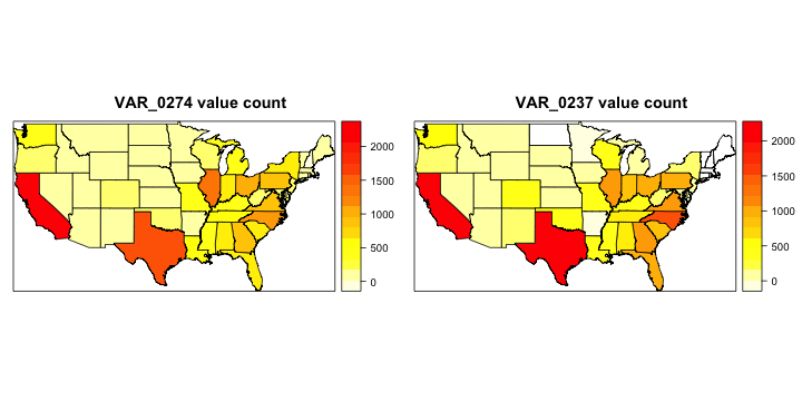
Goal: find the number of unique values per column.
So, now we have numerical feature, character features, and date features. We can calculate the number of unique values in each column of each set of features by running this function on the fly, length(unique(x)). Once we have all of the counts, we can row bind the vectors, which will make one big vector and tack on another column that describes the type of variable (numerical, character, date). Now we have a really long data frame with two columns called ‘all_ct’ that has the number of unique elements of each feature followed by the feature type.
Now to visualize this we can simply pass it through ggplot() and make histograms. Now IMO these graphs area little confusing. Because ggplot outputs the y-axis labeled ‘count’ and the variable we used to create the data frame ‘all_ct’ was called ‘count’. But remember the y-axis is just the number of features that has that many unique elements. Recall we read 20,000 rows of the train dataset, so the most unique elements a feature could have is 20,000 (or in the code it is called using ‘nrow(train)’)).
num_ct = sapply(train_numr, function(x) length(unique(x)))
char_ct = sapply(train_char, function(x) length(unique(x)))
date_ct = sapply(train_date, function(x) length(unique(x)))
all_ct = rbind(data.frame(count=num_ct, type="Numerical"),
               data.frame(count=char_ct, type="Character"),
               data.frame(count=date_ct, type="Date"))
# lets plot the unique values per feature
g1 = ggplot(all_ct, aes(x = count, fill=type)) +
   geom_histogram(binwidth = 1, alpha=0.7, position="identity") +
   xlab("Unique values per feature (0-100)")+ theme(legend.position = "none") +
   xlim(c(0,100)) +theme(axis.title.x=element_text(size=14, ,face="bold"))
g2 = ggplot(all_ct, aes(x = count, fill=type)) +
   geom_histogram(binwidth = 100, alpha=0.7, position="identity") +
   xlab("Unique values per feature(101+)")  + xlim(c(101,nrow(train))) +
   theme(axis.title.x=element_text(size=14, ,face="bold"))
grid.arrange(g1, g2, ncol=2)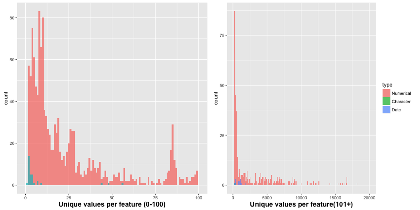
Here we pretty much do the same thing as the last chunk of code, but for NAs instead of unique values. As you can see on the graph, ‘breaks’ allows you to set the tick marks on the axis specified. We must ‘scale_x_log10’ if we actually want to see the data at these break marks because otherwise the x-axis would get too scrunched. If you want to see what I mean, try changing ‘scale_x_log10’ to ‘scale_x_continuous’. Our final result shows that most features have somewhere from 0 - 100 NA values.
num_na = sapply(train_numr, function(x) sum(is.na(x)))
char_na = sapply(train_char, function(x) sum(is.na(x)))
date_na = sapply(train_date, function(x) sum(is.na(x)))
all_na = rbind(data.frame(count=num_na, type="Numerical"),
               data.frame(count=char_na, type="Character"),
               data.frame(count=date_na, type="Date"))
#table(all_na)
all_na = data.frame(all_na)
all_na = all_na[all_na$count>0,]

breaks <- c(5,10,50,100,500,1000,2000)

ggplot(all_na, aes(x = count, fill=type)) +
  geom_histogram(alpha=0.7) +
#  scale_y_log10(limits=c(1,2000), breaks=breaks) +
  scale_x_log10(limits=c(1,20000), breaks=c(breaks,5000,10000,20000)) +
  labs(title="Histogram of feature count per NA count", size=24, face="bold") +
  theme(plot.title = element_text(size = 16, face = "bold")) +
  xlab("NA Count") + ylab("Feature Count")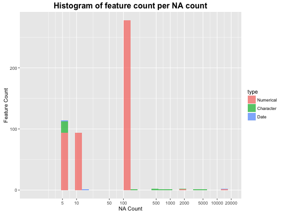
Goal: look at the numerical values.
The issue here is that most of the features are numerical…and there are A LOT. So instead of viewing all of them, we need to randomly sample them; we’ll take 100 of them (not a rigorously derived number, but…). The function sample() will do most of the work here by sampling values from 1 through the number of columns in the numerical training set. Then we will take the elements of ‘train_numr’ that fall in those spaces and save them to a new object ‘train_numr_samp’.
set.seed(200)
train_numr_samp = train_numr[,sample(1:ncol(train_numr),100)]
str(lapply(train_numr_samp[,sample(1:100)], unique))
## List of 100
## $ VAR_0194: int [1:4] 0 1 NA 3
## $ VAR_1230: int [1:5] 0 1 99 98 2
## $ VAR_1267: int [1:44] 9 2 8 3 6 4 1 16 5 99 ...
## $ VAR_1074: int [1:36] 0 11 1 5 7 2 6 8 999 3 ...
## $ VAR_1771: int [1:11] 0 97 1 99 98 5 2 3 4 7 ...
## $ VAR_1306: int [1:11] 0 97 1 2 99 98 3 4 5 6 ...
## $ VAR_1277: int [1:30] 2 4 1 0 6 3 9 99 98 8 ...
## $ VAR_1058: int [1:13] 0 3 1 2 99 5 4 6 8 7 ...
## $ VAR_0335: num [1:350] 0 1.04 0.2 0.67 2.74 1.11 0.35 0.28 -1 0.59 ...
## $ VAR_0373: int [1:5] 0 NA 1 2 3
## $ VAR_1389: int [1:27] 0 4 2 3 1 8 6 5 11 7 ...
## $ VAR_1387: int [1:31] 0 1 3 7 2 4 8 5 9 6 ...
## $ VAR_0626: int [1:10] 0 1 4 3 2 5 6 7 9 8
## $ VAR_1685: int [1:5231] 999999997 303472 94990 999999998 321783 999999996 145391 104442 999999999 208990 ...
## $ VAR_1325: int [1:9] 1 30 400 999 998 120 60 90 0
## $ VAR_1128: int [1:98] 100 56 92 13 11 83 20 67 57 0 ...
## $ VAR_0772: int [1:9] -99999 0 2 1 4 3 5 6 7
## $ VAR_1111: int [1:113] 994 0 999 100 997 20 11 10 2 19 ...
## $ VAR_1846: int [1:38] 999999998 999999999 999999997 999999996 6300 10080 16200 11940 630 12660 ...
## $ VAR_0065: int [1:118] 1 3 2 8 43 4 10 6 21 7 ...
## $ VAR_1579: int [1:201] 9 24 0 124 114 42 6 21 37 22 ...
## $ VAR_0019: int [1:2] 0 NA
## $ VAR_0646: int [1:28] 97 3 2 6 1 0 4 99 98 7 ...
## $ VAR_0461: int [1:10] 0 1 2 NA 3 5 6 4 10 7
## $ VAR_0615: int [1:62] 0 50 997 100 20 10 67 80 60 999 ...
## $ VAR_0317: int [1:6229] 64865 304500 0 126479 353211 120838 290689 81581 65000 22900 ...
## $ VAR_1841: int [1:565] 232 138 97 188 443 65 215 70 90 48 ...
## $ VAR_1923: int [1:642] 999999998 999999997 1900 999999996 999999999 6800 500 4000 1700 11600 ...
## $ VAR_0209: int [1:691] NA 583 492 113 486 948 6 676 648 698 ...
## $ VAR_1818: int [1:10] 994 1 30 999 998 997 60 400 120 90
## $ VAR_1088: int [1:9305] 0 2720 962 562005 21245 121 573 715 2985 75116 ...
## $ VAR_1318: int [1:721] 20000 300 999999996 600 500 700 1000 200 3000 2230 ...
## $ VAR_0444: int [1:629] 0 400 NA 437 2359 1496 1165 345 363 180 ...
## $ VAR_0949: int [1:85] 9998 9996 3 33 9999 30 49 47 54 20 ...
## $ VAR_0551: int [1:39] 9996 9999 34 82 18 44 17 55 1 47 ...
## $ VAR_0715: int [1:30] 1 2 -99999 0 3 5 8 4 10 9 ...
## $ VAR_0447: int [1:719] 0 1045 2698 NA 1176 1600 6786 1714 1761 891 ...
## $ VAR_0564: int [1:6] 0 2 1 4 3 6
## $ VAR_0696: int [1:36] 98 0 10 11 7 15 99 18 2 4 ...
## $ VAR_1802: int [1:8964] 49463 5296 999999997 2060 13576 1237 143 350 3739 1197 ...
## $ VAR_0357: int [1:10] 1 0 2 4 3 NA 5 6 7 10
## $ VAR_0911: int [1:42] 97 0 1 6 5 2 4 99 8 3 ...
## $ VAR_1112: int [1:142] 994 67 100 95 9 0 49 23 999 29 ...
## $ VAR_1110: int [1:167] 66 99 88 77 59 75 98 83 92 46 ...
## $ VAR_0313: int [1:8505] 0 163400 127200 252970 33850 813900 36350 46000 21536 57870 ...
## $ VAR_0719: int [1:37] 1 2 4 3 0 8 9 6 5 7 ...
## $ VAR_0879: int [1:93] 11 57 0 13 54 75 9 20 10 67 ...
## $ VAR_1762: int [1:37] 2 8 0 1 3 16 4 7 99 98 ...
## $ VAR_0758: int [1:22] 0 1 7 2 3 6 4 5 8 19 ...
## $ VAR_1077: int [1:35] 0 2 3 4 999 1 12 5 15 8 ...
## $ VAR_1134: int [1:85] 9996 24 0 6 3 2 7 64 17 22 ...
## $ VAR_0494: int [1:8] 0 -1 2 3 4 NA 1 5
## $ VAR_0898: int [1:8287] 49463 5432 -99999 183 10325 1829 116 219 412 1501 ...
## $ VAR_1257: int [1:10] 1 30 400 0 999 998 60 997 90 120
## $ VAR_1767: int [1:40] 2 8 97 0 9 1 5 3 17 4 ...
## $ VAR_0435: int [1:307] 0 49932 38088 NA 1216929 7195 6909 24267 12402 22914 ...
## $ VAR_1215: int [1:309] 999999998 999999997 999999999 10167 4226 11097 12780 999999996 11299 9085 ...
## $ VAR_0995: int [1:5] 0 1 99 2 3
## $ VAR_1082: int [1:16750] 76857 341365 107267 47568 23647 21139 327744 4326 27128 1197 ...
## $ VAR_1379: int [1:10] 1 30 400 60 120 999 998 0 90 997
## $ VAR_0853: int [1:129] -99999 1 26 3 6 5 0 10 14 22 ...
## $ VAR_0340: int [1:3995] -1 107771 26025 -23464 21900 128706 -71077 64726 64948 138705 ...
## $ VAR_1151: int [1:85] 9996 38 53 26 37 10 27 32 9 35 ...
## $ VAR_0655: int [1:1670] 999999997 604 0 129 691 587 420 264 1052 999999996 ...
## $ VAR_0322: int [1:445] 181 25 118 100 138 15 58 17 77 30 ...
## $ VAR_1433: int [1:6] 98 97 99 0 1 2
## $ VAR_1161: int [1:18] 0 1 2 4 7 5 3 13 6 25 ...
## $ VAR_1283: int [1:17] 0 97 2 99 98 1 4 3 6 5 ...
## $ VAR_1142: int [1:83] 9996 2 1 9999 7 12 32 35 25 8 ...
## $ VAR_1463: int [1:30] 97 3 2 8 1 0 4 99 98 5 ...
## $ VAR_0259: int [1:4] 0 1 NA 2
## $ VAR_1525: int [1:86] 9996 24 23 0 2 80 17 22 12 9999 ...
## $ VAR_0964: int [1:2314] 999999997 999999998 20662 999999996 1806 3740 3632 129873 999999999 2015 ...
## $ VAR_0379: int [1:4] 0 NA 1 2
## $ VAR_0333: int [1:4907] 0 176154 65600 68120 82700 61600 537050 41300 45000 21600 ...
## $ VAR_0846: int [1:20] -99999 0 1 3 7 2 6 4 5 8 ...
## $ VAR_0066: int [1:71] 0 1 5 7 12 15 6 27 2 4 ...
## $ VAR_0134: int [1:24] 0 2 4 1 6 12 5 3 10 8 ...
## $ VAR_0289: int [1:1362] -1 165000 141950 35000 6800000 130500 106615 66500 283500 175000 ...
## $ VAR_0947: int [1:9] 98 1 0 97 99 96 2 3 4
## $ VAR_0849: int [1:26] 5 1 0 2 3 10 14 16 7 -99999 ...
## $ VAR_1384: int [1:565] 232 138 97 188 443 65 215 70 90 48 ...
## $ VAR_0768: int [1:34] 0 5 15 1 3 2 4 8 6 11 ...
## $ VAR_0904: int [1:418] -99999 10200 7000 5000 2500 1200 500 3500 3000 5001 ...
## $ VAR_1877: int [1:37] 1 5 2 3 98 0 4 14 8 99 ...
## $ VAR_1092: int [1:1112] 0 100 999999999 6301 999999997 1662 25 650 2356 8375 ...
## $ VAR_1916: int [1:8] 998 1 400 999 120 90 60 30
## $ VAR_0541: int [1:15412] 49463 303472 94990 20593 10071 18877 321783 2961 20359 815 ...
## $ VAR_1351: int [1:14] 0 1 97 2 99 98 4 6 3 5 ...
## $ VAR_1628: int [1:155] 999999997 0 999999998 999999999 2443 928 1505 1631 7162 3805 ...
## $ VAR_0601: int [1:135] 997 998 999 996 995 8 3 39 42 50 ...
## $ VAR_0546: int [1:8] 998 1 400 999 30 120 90 60
## $ VAR_1251: int [1:372] 0 999999997 100 999999999 999999998 25 275 167 999999996 900 ...
## $ VAR_1035: int [1:40] 0 1 6 3 2 5 7 4 9 12 ...
## $ VAR_0327: int [1:4] 0 1 -1 NA
## $ VAR_0212: num [1:18198] NA 9.21e+10 2.65e+10 7.76e+10 6.04e+10 ...
## $ VAR_1466: int [1:11] 97 0 1 99 98 2 3 4 5 6 ...
## $ VAR_1270: int [1:10] 0 1 99 98 3 2 4 5 6 7
## $ VAR_1266: int [1:300] 113 78 84 76 122 27 90 61 48 13 ...
## [list output truncated]We reshape ‘train_numr_samp’ to replace all NA values with the numerical value -99999999. ‘is.na’ just creates a long boolean vector where all of the TRUE values are the NAs and we assign them this new numerical value instead.
Second line of below chunk reads, how many columns from train_numr contain all the same value. Because we know that if the variance is equal to 0 then we must have a column of all the same value. Our new function built on the fly passes over the columns of train_numr and calculates the variance without the NA values. So there are 41 features with no unique values.
train_numr_samp[is.na(train_numr_samp)] = -99999999
length(colnames(train_numr[,sapply(train_numr, function(v) var(v, na.rm=TRUE)==0)]))
## [1] 41‘dev.off()’ just stands for ‘device off’. You’ll notice when you run it that your plot will disappear. It’s important to use when you are saving .png’s or .jpg’s or the sort.
## RStudioGD
##         2
cor() creates a massive correlation matrix where each element is the correlation between that variable and another. This matrix can then be passed to a function that graphs it in a second.
corrplot() accepts the cor() matrix as input to put out a nice plot of the correlation between each variable. The first plot uses Pearson correlation. If you’ve taken some stats this is the little r value that you square to get big $R^2$ (used in linear relationships). It’s also the default method of the function cor(). On the plot we can see that all of the diagonal spaces are dark blue, this is just because each variable is 100% correlated with itself. The second plot uses Spearman correlation. It’s always good practice to run both Pearson and Spearman because Pearson deals with linear relationships so it may falter in some non-linear scenarios where Spearman might do better. If we have a situation where the Spearman is greater than the Pearson, this certainly indicates that there is something non-linear going on and we may need a log transform on a variable or more. tl.pos=”n” means don’t add text labels, trust me this is necessary. You don’t want the label to every variable on this graph (if you don’t believe me set this to “d”). order = “hclust” refers to how the variables are ordered when they are plotted. In this case, it is a heirarchical clustering order. We don’t need to worry too much about this, but it essentially means that the most similar variables are joined one-by-one until they are all joined together. Or in other words, the most similar ones are together. You can play around with this value if you want to see other orderings of the plot.
#compute the correlation matrix
descrCor_pear <-  cor(scale(train_numr_samp,center=TRUE,scale=TRUE), method="pearson")
descrCor_spea <-  cor(scale(train_numr_samp,center=TRUE,scale=TRUE), method="spearman")
# Kendall takes too long to run
# descrCor_kend <-  cor(scale(train_numr_samp,center=TRUE,scale=TRUE), method="kendall")
#visualize the matrix, clustering features by correlation index.
corrplot(descrCor_pear, order = "hclust", mar=c(0,0,1,0), tl.pos="n", main="Pearson correlation of 100 sampled numerical features")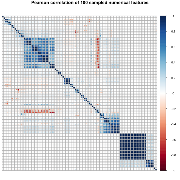
corrplot(descrCor_spea, order = "hclust", mar=c(0,0,1,0), tl.pos="n", main="Spearman correlation of 100 sampled numerical features")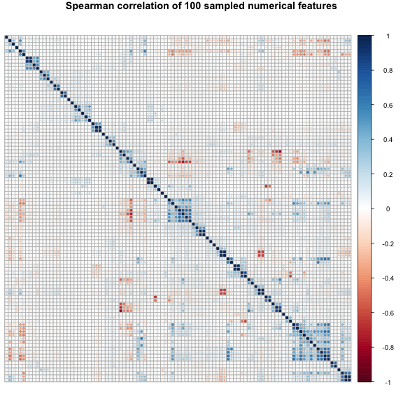
Goal: create a plot that shows the proportion of features containing a max correlation to another feature below each correlation threshold.
expand.grid() creates a data frame from all combinations of the vectors or factors you give it. In our case we are giving the function 3 arguments, two of which are NA for now, and the corr_limit is just the sequence from 0 to 1 by 0.01. findCorrelation() runs through a correlation matrix and gives you the columns to remove to reduce pair-wise correlations. This is often used for feature selection. So we want the number of columns to remove from both ‘descrCor_pear’ and ‘descrCor_spea’ for every possible correlation cutoff in corr_limit. This number ends up, conveniently, being a percentage since we sampled 100 numerical features. We can imagine that for very low correlation cutoffs most of the features will be removed, and vice versa. Then for each of these values we will save them in the vector columns we created ‘perc_feat_pear’ and ‘perc_feat_spea’.
Now we just plot. The first plot() builds the plot itself (axes, etc.), and the abline() creates the dashed background lines. The two points() calls place the actual points on the graph. (Really the pearson points are being placed twice because they were also called in the initial plot() function). At a corr_limit of 0.00 99 of the 100 features are told to be removed by findCorrelation() for both Pearson and Spearman. At a corr_limit of 0.99, 22 Pearson features are to be removed and 1 Spearman feature. This is why we have to take (100 - corr.df$perc_feat_pear) to get the % value we want.
corr.df = expand.grid(corr_limit=(0:100)/100, perc_feat_pear=NA, perc_feat_spea=NA)
for(i in 0:100){
  corr.df$perc_feat_pear[i+1]=length(findCorrelation(descrCor_pear, i/100))
  corr.df$perc_feat_spea[i+1]=length(findCorrelation(descrCor_spea, i/100))
}

plot(corr.df$corr_limit, abs(100-corr.df$perc_feat_pear), pch=19, col="blue",
     ylab = "Feature % falling below abs(correlation)", xlab="Absolute Correlation",
     main="Cumulative distribution of correlation\n(Within 100 sampled numerical features)")
abline(h=(0:10)*10, v=(0:20)*.05, col="gray", lty=3)
points(corr.df$corr_limit, abs(100-corr.df$perc_feat_pear), pch=19, col="blue")
points(corr.df$corr_limit, abs(100-corr.df$perc_feat_spea), pch=19, col="red")
legend("topleft", c("Pearson", "Spearman"), col = c("blue", "red"), pch = 19, bg="white")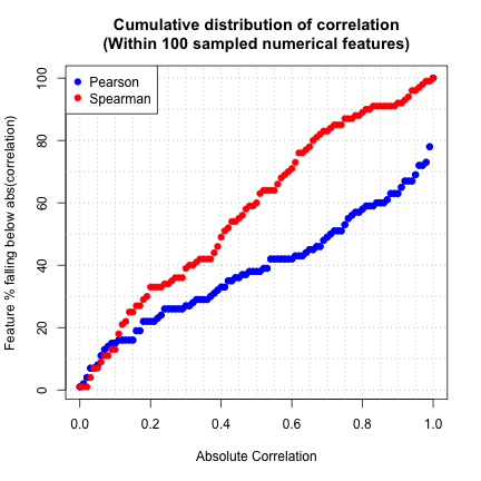
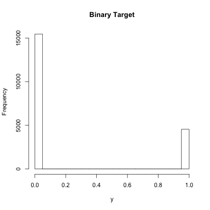
Recall, at the very beginning we saved train$target as the varaible ‘y’. So here we can take a look at this target variable, which is binary.
hist(y, main="Binary Target")