Apologies for the small gap in posts here, between a change in dwelling and a lost computer due to an unoftunate crash I have been away for a bit. But I’m back. Where would I be without a couple of upgrades, so after a short wait period I’ve received my new machine and ready to get back to annotatoR.
This is the most popoular script on Kaggle. It is another exploratory analysis, but this time on Rossmann Store Sales. The author of the script, Christian Thiele, has some comments which I have left in surrounded by quotes. Keep in mind the goal of the competition is to predict 6 weeks of daily sales for 1,115 stores located across Germany.
“This is an exploratory analysis of the Rossmann Store Sales data which can be found here. The data isn’t huge but the speedup using data.table is noticeable. It is nice to have unmasked data which allows for some interpretations.”
When you download the data, if you are using the same script, you must make a folder as your working directory and within that folder make a folder called “input” and then place the data in there. We can see below that the script reads the data into R through the directory “input”. (Directory and folder are the same thing)
Goal: “Read in the data:”
library(data.table)
library(zoo)
library(forecast)
library(ggplot2)
test <- fread("input/test.csv")
train <- fread("input/train.csv")
store <- fread("input/store.csv")
“Let’s have a first look at the data:”
Goal: first explorations of datasets
str() is always a great method for viewing your data quickly and efficiently. You really get the most information about the variables, like, how they are classified by R (this is a big one as sometimes variables can seem like int but actually are chr, or something), the variable names, and the first several entries within the column. After using str() we can also use head() and tail() which gives the first and last 6 rows, respectively. This feels like a better way to see how the data are structures (personally), but does not tell you how R is reading each variable. You can also add a number after train, such as, head(train, 20), to get the first 20 rows.
After viewing the data, we don’t want the dates to be character strings. We want the dates to be read as dates by R. So we take the Date column of train and set it to be read as such using as.Date(). This is done with the train dataset and the test dataset. Now if you go back and look at str(train) you will see that the Date column is now classified as “Date, format:”. Same with the test dataframe. Since R now reads the dates as actual dates instead of character strings we can order the whole datset according to the dates, from earliest to most recent. This action is done using the “train <- train[order(Date)]” line. This essentially says, order the column Date and then reorder all of the rows of train in that same order, then reassign the name “train” to this new dataframe. The summary() command tells us that there exist 11 NAs in the test dataframe (Christian Thiele notes this below). So we run “test[is.na(test\$Open), ]” and we see that only store 622 has NA values and they all exist in the “Open” column. So we isolate those NA values within the Open column using “test\$Open[test\$Store == 622]”, which says to take only elements of test\$Open where the Store is 622.
str(train)## Classes 'data.table' and 'data.frame': 1017209 obs. of 9 variables:
## $ Store : int 1 2 3 4 5 6 7 8 9 10 ...
## $ DayOfWeek : int 5 5 5 5 5 5 5 5 5 5 ...
## $ Date : chr "2015-07-31" "2015-07-31" "2015-07-31" "2015-07-31" ...
## $ Sales : int 5263 6064 8314 13995 4822 5651 15344 8492 8565 7185 ...
## $ Customers : int 555 625 821 1498 559 589 1414 833 687 681 ...
## $ Open : int 1 1 1 1 1 1 1 1 1 1 ...
## $ Promo : int 1 1 1 1 1 1 1 1 1 1 ...
## $ StateHoliday : chr "0" "0" "0" "0" ...
## $ SchoolHoliday: chr "1" "1" "1" "1" ...
## - attr(*, ".internal.selfref")=<externalptr>str(test)## Classes 'data.table' and 'data.frame': 41088 obs. of 8 variables:
## $ Id : int 1 2 3 4 5 6 7 8 9 10 ...
## $ Store : int 1 3 7 8 9 10 11 12 13 14 ...
## $ DayOfWeek : int 4 4 4 4 4 4 4 4 4 4 ...
## $ Date : chr "2015-09-17" "2015-09-17" "2015-09-17" "2015-09-17" ...
## $ Open : int 1 1 1 1 1 1 1 1 1 1 ...
## $ Promo : int 1 1 1 1 1 1 1 1 1 1 ...
## $ StateHoliday : chr "0" "0" "0" "0" ...
## $ SchoolHoliday: chr "0" "0" "0" "0" ...
## - attr(*, ".internal.selfref")=<externalptr>str(store)## Classes 'data.table' and 'data.frame': 1115 obs. of 10 variables:
## $ Store : int 1 2 3 4 5 6 7 8 9 10 ...
## $ StoreType : chr "c" "a" "a" "c" ...
## $ Assortment : chr "a" "a" "a" "c" ...
## $ CompetitionDistance : int 1270 570 14130 620 29910 310 24000 7520 2030 3160 ...
## $ CompetitionOpenSinceMonth: int 9 11 12 9 4 12 4 10 8 9 ...
## $ CompetitionOpenSinceYear : int 2008 2007 2006 2009 2015 2013 2013 2014 2000 2009 ...
## $ Promo2 : int 0 1 1 0 0 0 0 0 0 0 ...
## $ Promo2SinceWeek : int NA 13 14 NA NA NA NA NA NA NA ...
## $ Promo2SinceYear : int NA 2010 2011 NA NA NA NA NA NA NA ...
## $ PromoInterval : chr "" "Jan,Apr,Jul,Oct" "Jan,Apr,Jul,Oct" "" ...
## - attr(*, ".internal.selfref")=<externalptr># head(train); tail(train)
# head(test); tail(test)
train[, Date := as.Date(Date)]
test[, Date := as.Date(Date)]
# storetrain <- train[order(Date)]
test <- test[order(Date)]
summary(train)## Store DayOfWeek Date Sales
## Min. : 1.0 Min. :1.000 Min. :2013-01-01 Min. : 0
## 1st Qu.: 280.0 1st Qu.:2.000 1st Qu.:2013-08-17 1st Qu.: 3727
## Median : 558.0 Median :4.000 Median :2014-04-02 Median : 5744
## Mean : 558.4 Mean :3.998 Mean :2014-04-11 Mean : 5774
## 3rd Qu.: 838.0 3rd Qu.:6.000 3rd Qu.:2014-12-12 3rd Qu.: 7856
## Max. :1115.0 Max. :7.000 Max. :2015-07-31 Max. :41551
## Customers Open Promo StateHoliday
## Min. : 0.0 Min. :0.0000 Min. :0.0000 Length:1017209
## 1st Qu.: 405.0 1st Qu.:1.0000 1st Qu.:0.0000 Class :character
## Median : 609.0 Median :1.0000 Median :0.0000 Mode :character
## Mean : 633.1 Mean :0.8301 Mean :0.3815
## 3rd Qu.: 837.0 3rd Qu.:1.0000 3rd Qu.:1.0000
## Max. :7388.0 Max. :1.0000 Max. :1.0000
## SchoolHoliday
## Length:1017209
## Class :character
## Mode :character
##
##
## summary(test)## Id Store DayOfWeek Date
## Min. : 1 Min. : 1.0 Min. :1.000 Min. :2015-08-01
## 1st Qu.:10273 1st Qu.: 279.8 1st Qu.:2.000 1st Qu.:2015-08-12
## Median :20544 Median : 553.5 Median :4.000 Median :2015-08-24
## Mean :20544 Mean : 555.9 Mean :3.979 Mean :2015-08-24
## 3rd Qu.:30816 3rd Qu.: 832.2 3rd Qu.:6.000 3rd Qu.:2015-09-05
## Max. :41088 Max. :1115.0 Max. :7.000 Max. :2015-09-17
##
## Open Promo StateHoliday SchoolHoliday
## Min. :0.0000 Min. :0.0000 Length:41088 Length:41088
## 1st Qu.:1.0000 1st Qu.:0.0000 Class :character Class :character
## Median :1.0000 Median :0.0000 Mode :character Mode :character
## Mean :0.8543 Mean :0.3958
## 3rd Qu.:1.0000 3rd Qu.:1.0000
## Max. :1.0000 Max. :1.0000
## NA's :11test[is.na(test$Open), ] # Only store 622## Id Store DayOfWeek Date Open Promo StateHoliday SchoolHoliday
## 1: 10752 622 6 2015-09-05 NA 0 0 0
## 2: 9040 622 1 2015-09-07 NA 0 0 0
## 3: 8184 622 2 2015-09-08 NA 0 0 0
## 4: 7328 622 3 2015-09-09 NA 0 0 0
## 5: 6472 622 4 2015-09-10 NA 0 0 0
## 6: 5616 622 5 2015-09-11 NA 0 0 0
## 7: 4760 622 6 2015-09-12 NA 0 0 0
## 8: 3048 622 1 2015-09-14 NA 1 0 0
## 9: 2192 622 2 2015-09-15 NA 1 0 0
## 10: 1336 622 3 2015-09-16 NA 1 0 0
## 11: 480 622 4 2015-09-17 NA 1 0 0test$Open[test$Store == 622]## [1] 1 0 1 1 1 1 1 1 0 1 1 1 1 1 1 0 1 1 1 1 1 1 0
## [24] 1 1 1 1 1 1 0 1 1 1 1 1 NA 0 NA NA NA NA NA NA 0 NA NA
## [47] NA NA“The test set has just 41088 rows while the train set has 1017209 rows.
The public leaderboard is based on 39% of the data (16024 rows) and the private leaderboard
is based on 61% of the data (25064 rows). Store 622 has 11 missing values in the
Open columns, but not all of the data in that column of that store is missing.
As was pointed out here it should probably be imputed as 1.”
“Additionally, the whole Customers column is missing from the test data (since
that data is only known ex post).”
test[is.na(test)] <- 1Goal: look closer at the differences between test and train
.SD is like a subset of data.table. It is typically used to run a function through the columns of a data.table while subsetting based on another column. You can see what I mean by running something like: “train[, lapply(.SD, function(x) length(unique(x))), by = “DayOfWeek”]” instead. But without subsetting based on another column, we simply run the unique() function through the columns and return the number of unique values for each. As you can see, the test set has 41088 rows and 41088 unique ID values, which makes sense.
“sum(unique(test\$Store) %in% unique(train\$Store))” asks the data how many of the stores in the test dataframe are in the train dataframe. The answer is all of them. We then ask the same question, but the other way around, and we see that 259 stores in the train dataframe are not in the test dataframe. This is shown by the ! - exclamation point, indicating “the opposite, or not”. We then just check some percentages indicating how often each factor variable occurs. table() builds a small table of counts at each factor level.
“During the test period there are no Easter or Christmas holidays but interestingly during a rather large portion of the time (44%) there are school holidays while that is the case for only 18% of the train data:”
# Unique values per column
train[, lapply(.SD, function(x) length(unique(x)))]
## Store DayOfWeek Date Sales Customers Open Promo StateHoliday
## 1: 1115 7 942 21734 4086 2 2 4
## SchoolHoliday
## 1: 2test[, lapply(.SD, function(x) length(unique(x)))]## Id Store DayOfWeek Date Open Promo StateHoliday SchoolHoliday
## 1: 41088 856 7 48 2 2 2 2# All test stores are also in the train data
sum(unique(test$Store) %in% unique(train$Store))## [1] 856# 259 train stores are not in the test data
sum(!(unique(train$Store) %in% unique(test$Store)))## [1] 259table(train$Open) / nrow(train) # Percent Open Train##
## 0 1
## 0.1698933 0.8301067table(test$Open) / nrow(test) # Percent Open Test ##
## 0 1
## 0.1456386 0.8543614table(train$Promo) / nrow(train) # Percent of the time promo in train##
## 0 1
## 0.6184855 0.3815145table(test$Promo) / nrow(test) # Percent of the time promo in test##
## 0 1
## 0.6041667 0.3958333table(train$StateHoliday) / nrow(train) # Percent of the time holiday in train##
## 0 a b c
## 0.969475300 0.019917244 0.006576820 0.004030637table(test$StateHoliday) / nrow(test) # no b and c = no easter holiday and no christmas##
## 0 a
## 0.995619159 0.004380841table(train$SchoolHoliday) / nrow(train) # Percent of the time school holiday in train##
## 0 1
## 0.8213533 0.1786467table(test$SchoolHoliday) / nrow(test) # Percent of the time school holiday in test##
## 0 1
## 0.5565129 0.4434871“There are no obvious breaks in the data. The test period ranges from 2015-08-01 to 2015-09-17, so the task is to predict 48 days. The train period ranges from 2013-01-01 to 2015-07-31.” The plots below show that there are no obvious breaks in the data because there would be a hole in the graph. We then ask if all 856 stores exist within each day, and this can be verified if all() responds TRUE because it would indicate that every logical response within the argument is a TRUE value.
plot(train$Date, type = "l")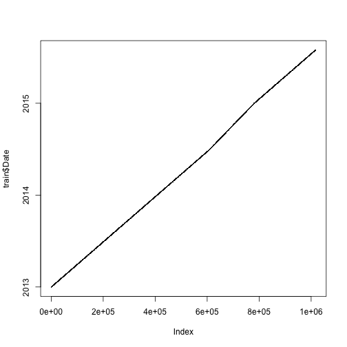
plot(test$Date, type = "l")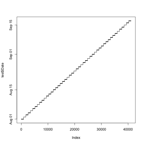
# As expected all 856 stores to be predicted daily
all(table(test$Date) == 856)
## [1] TRUERecall that the test dataframe does not contain the columns “Sales” and “Customers”, only the train dataframe has this data. “Let’s look at the columns that are unique to the train set:”
Goal: visualize the two variables in train but not in test
First, we look at a histogram of the Sales using 100 breaks for the histogram bins.
It would make sense to look at the Sales on only the days that the store was not closed. To do this, we can take only the elements within the Sales column of train where Sales is != (not equal to) 0, and return summary statistics grouped by a certain feature using aggregate(). This is an interesting way of calling those days when the store is not closed because of course there would be some sale or customer if the store is open, I would hope. In this case, the summary statistic is “mean” and the feature is the stores. So we get an average across the individual store.
hist(train$Sales, 100)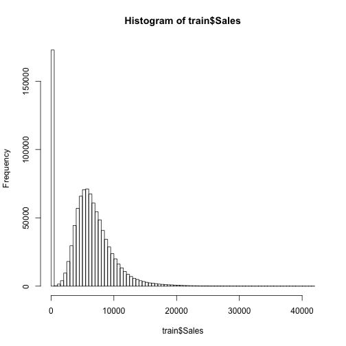
hist(aggregate(train[Sales != 0]$Sales,
               by = list(train[Sales != 0]$Store), mean)$x, 100,
     main = "Mean sales per store when store was not closed")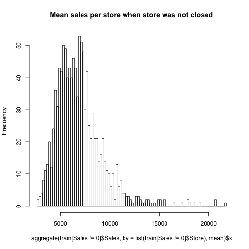
Then we look at the same two histograms for the customers.
hist(train$Customers, 100)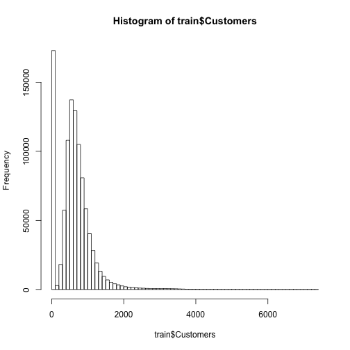
hist(aggregate(train[Sales != 0]$Customers,
               by = list(train[Sales != 0]$Store), mean)$x, 100,
     main = "Mean customers per store when store was not closed")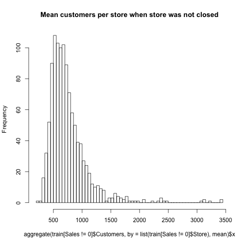
ggplot() gives a wide range of plotting possibilities, which have been documented to death in many resources available online or by Hadley Wickham. The gist of it is that you call ggplot() function on some data, and then the aes() argument tells it the mapping values (x-axis, y-axis), and then you use + signs to change the formatting of the coordinate system (size, shape, color, etc.). I would suggest checking out the ggplot2 cheat sheet for quick reference. The data that we are using for each graph is the same data from the histograms earlier, Sales and Customers when the store is open. The ampersand is an important addition because this means that only the data where sales and customers are not equal to zero are used. factor() temporarily forces that variable to be a factor variable, where R creates dummy variables for each factor level and evaluates at those levels rather than continuously.
ggplot(train[Sales != 0], aes(x = factor(SchoolHoliday), y = Sales)) +
    geom_jitter(alpha = 0.1) +
    geom_boxplot(color = "yellow", outlier.colour = NA, fill = NA)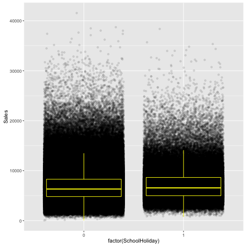
ggplot(train[train$Sales != 0 & train$Customers != 0],
       aes(x = log(Customers), y = log(Sales))) +
    geom_point(alpha = 0.2) + geom_smooth()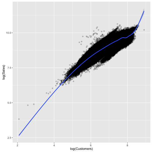
ggplot(train[train$Sales != 0 & train$Customers != 0],
       aes(x = factor(Promo), y = Sales)) +
    geom_jitter(alpha = 0.1) +
    geom_boxplot(color = "yellow", outlier.colour = NA, fill = NA)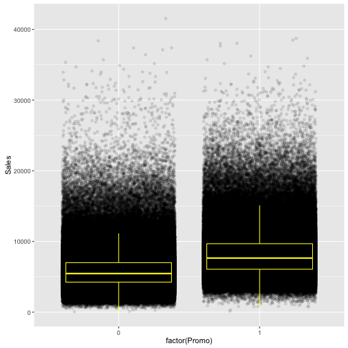
ggplot(train[train$Sales != 0 & train$Customers != 0],
       aes(x = factor(Promo), y = Customers)) +
    geom_jitter(alpha = 0.1) +
    geom_boxplot(color = "yellow", outlier.colour = NA, fill = NA)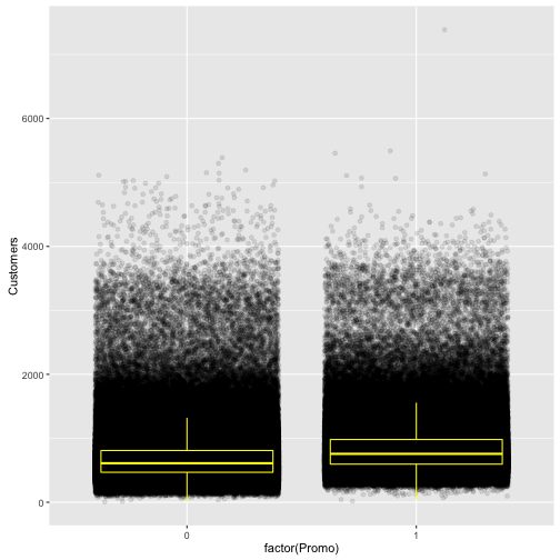
“Note: I chose to not plot that data including days with 0 sales or customers because that would have biased the boxplots.”
It surprises me that there exists data that has sales but no customers or vice versa. If there are days with sales but no customers, this is a data provenance issue and the author deals with this appropriately by only taking those days where sales and customers are not 0.
“Sales is as expected strongly correlated with the number of customers. It looks like the Boxplots of customers overlap a little more than the boxplots of sales. This would mean that the promos are not mainly attracting more customers but make customers spend more. The mean amount spent per customer is about one Euro higher:”
Goal: are promos effective?
The with() function first takes some data, and then an expression to apply to that data. So in this case we apply the mean(Sales / Customers) to those data where Sales is not 0 and break it up between whether or not a Promo was going on.
with(train[train$Sales != 0 & train$Promo == 0], mean(Sales / Customers))## [1] 8.941128with(train[train$Sales != 0 & train$Promo == 1], mean(Sales / Customers))## [1] 10.17896“There are sometimes promos while the respective store is closed and there are promos 45% of the time:”
ifelse() takes a logical statement, and then when it is true it outputs the second argument and when it is false it outputs the third argument.
table(ifelse(train$Sales != 0, "Sales > 0", "Sales = 0"),
      ifelse(train$Promo, "Promo", "No promo"))
##
## No promo Promo
## Sales = 0 161666 11205
## Sales > 0 467463 376875“At least there are no sales when the stores are closed but there are some stores that, according to the data, made no sales although they were opened even if they had some customers. These observations may be errors in the data / outliers:”
So this is what I was talking about earlier regarding data provenance. This is quite odd, but possible. Again we have a table of ifelse() functions and then we look at some data using the ampersand logical operator (when the store is open and there are no sales).
table(ifelse(train$Open == 1, "Opened", "Closed"),
      ifelse(train$Sales > 0, "Sales > 0", "Sales = 0"))
##
## Sales = 0 Sales > 0
## Closed 172817 0
## Opened 54 844338# That tends to happen on consecutive days. Some stores even had customers
# (who bought nothing?)
train[Open == 1 & Sales == 0]## Store DayOfWeek Date Sales Customers Open Promo StateHoliday
## 1: 762 4 2013-01-17 0 0 1 0 0
## 2: 232 4 2013-01-24 0 0 1 1 0
## 3: 339 3 2013-01-30 0 0 1 0 0
## 4: 339 4 2013-01-31 0 0 1 0 0
## 5: 259 4 2013-02-07 0 0 1 1 0
## 6: 353 6 2013-03-16 0 0 1 0 0
## 7: 948 4 2013-04-25 0 5 1 1 0
## 8: 589 1 2013-04-29 0 0 1 1 0
## 9: 364 2 2013-05-07 0 0 1 0 0
## 10: 364 3 2013-05-08 0 0 1 0 0
## 11: 681 5 2013-05-10 0 0 1 0 0
## 12: 700 3 2013-06-05 0 0 1 1 0
## 13: 665 5 2013-06-28 0 0 1 0 0
## 14: 665 6 2013-06-29 0 0 1 0 0
## 15: 1039 2 2013-07-09 0 0 1 0 0
## 16: 1039 3 2013-07-10 0 0 1 0 0
## 17: 927 4 2013-08-08 0 0 1 0 0
## 18: 391 3 2013-08-28 0 0 1 1 0
## 19: 663 1 2013-09-02 0 0 1 0 0
## 20: 983 5 2014-01-17 0 0 1 0 0
## 21: 983 6 2014-01-18 0 0 1 0 0
## 22: 623 5 2014-01-24 0 0 1 1 0
## 23: 623 6 2014-01-25 0 0 1 0 0
## 24: 25 3 2014-02-12 0 0 1 0 0
## 25: 25 4 2014-02-13 0 0 1 0 0
## 26: 327 3 2014-03-12 0 0 1 0 0
## 27: 986 2 2014-03-18 0 0 1 1 0
## 28: 850 6 2014-03-29 0 0 1 0 0
## 29: 661 5 2014-04-04 0 0 1 1 0
## 30: 1100 2 2014-04-29 0 3 1 1 0
## 31: 1100 3 2014-04-30 0 0 1 1 0
## 32: 1017 3 2014-06-04 0 0 1 1 0
## 33: 1017 4 2014-06-05 0 0 1 1 0
## 34: 57 2 2014-07-01 0 0 1 1 0
## 35: 925 4 2014-07-03 0 0 1 1 0
## 36: 102 6 2014-07-12 0 0 1 0 0
## 37: 882 3 2014-07-23 0 0 1 0 0
## 38: 887 3 2014-07-23 0 0 1 0 0
## 39: 102 4 2014-07-24 0 0 1 0 0
## 40: 238 4 2014-07-24 0 0 1 0 0
## 41: 303 4 2014-07-24 0 0 1 0 0
## 42: 387 4 2014-07-24 0 0 1 0 0
## 43: 28 2 2014-09-02 0 0 1 1 0
## 44: 28 3 2014-09-03 0 0 1 1 0
## 45: 28 4 2014-09-04 0 0 1 1 0
## 46: 548 5 2014-09-05 0 0 1 1 0
## 47: 835 3 2014-09-10 0 0 1 0 0
## 48: 227 4 2014-09-11 0 0 1 0 0
## 49: 835 4 2014-09-11 0 0 1 0 0
## 50: 357 1 2014-09-22 0 0 1 0 0
## 51: 708 3 2014-10-01 0 0 1 1 0
## 52: 699 4 2015-02-05 0 0 1 1 0
## 53: 674 4 2015-03-26 0 0 1 0 0
## 54: 971 5 2015-05-15 0 0 1 0 0
## Store DayOfWeek Date Sales Customers Open Promo StateHoliday
## SchoolHoliday
## 1: 0
## 2: 0
## 3: 0
## 4: 0
## 5: 0
## 6: 0
## 7: 0
## 8: 0
## 9: 0
## 10: 0
## 11: 0
## 12: 0
## 13: 0
## 14: 0
## 15: 0
## 16: 0
## 17: 1
## 18: 1
## 19: 1
## 20: 0
## 21: 0
## 22: 0
## 23: 0
## 24: 0
## 25: 0
## 26: 0
## 27: 0
## 28: 0
## 29: 0
## 30: 0
## 31: 0
## 32: 0
## 33: 0
## 34: 0
## 35: 0
## 36: 0
## 37: 1
## 38: 0
## 39: 1
## 40: 1
## 41: 1
## 42: 1
## 43: 1
## 44: 1
## 45: 0
## 46: 1
## 47: 0
## 48: 0
## 49: 0
## 50: 0
## 51: 0
## 52: 0
## 53: 0
## 54: 1
## SchoolHoliday“The stores have different amounts of days with zero sales. There are spikes in the sales before the stores close and after the reopen:”
sort() simply takes the data and orders them in ascending (default) or descending order. Here we are sorting the Sales data for each store with how many days have 0 sales. This is done using tapply(). There are a bunch of apply() functions. tapply() is typically used when you want to apply a function to data by groups. Here the groups are each store. Writing function(x) sum(x == 0) defines a function ‘on the fly’ and applies this function to all data in train\$Sales grouping by train\$Store. The sum() allows each of the days where sales were 0 to be counted and then the output is simply the number of total days with 0 sales for that store. The index for tapply() must be a list of factors, so train\$Store was coerced to a list using the list() function. Then this was all saved to the object zerosPerStore, which ends as an array.
train[Store == 972, Sales] means take the element of train where Store is 972 and then output the Sales column.
zerosPerStore <- sort(tapply(train$Sales, list(train$Store), function(x) sum(x == 0)))
hist(zerosPerStore,100)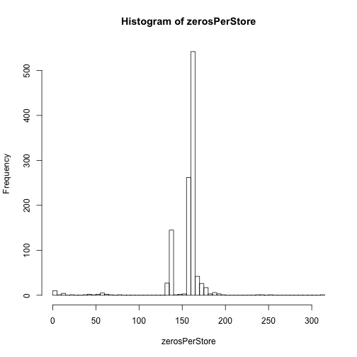
# Stores with the most zeros in their sales:
tail(zerosPerStore, 10)
## 105 339 837 25 560 674 972 349 708 103
## 188 188 191 192 195 197 240 242 255 311# Some stores were closed for some time, some of those were closed multiple times
plot(train[Store == 972, Sales], ylab = "Sales", xlab = "Days", main = "Store 972")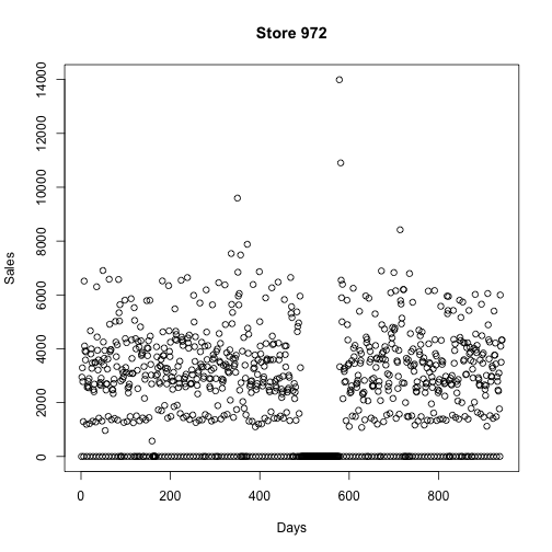
plot(train[Store == 103, Sales], ylab = "Sales", xlab = "Days", main = "Store 103")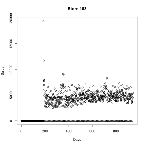
plot(train[Store == 708, Sales], ylab = "Sales", xlab = "Days", main = "Store 708")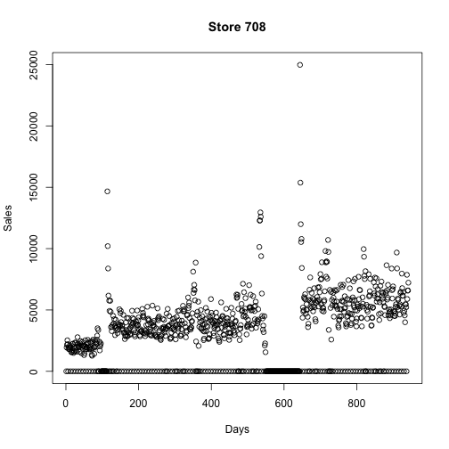
“There are also stores that have no zeros in their sales. These are the exception since they are opened also on sundays / holidays. The sales of those stores on sundays are particularly high:”
I must assume that the author here looked at a couple of days before just showing Sunday. But the intuition is obvious; a store that is never closed is probably a popular store and especially on weekends. The author also decided to omit the line of code where he tracked down those stores with zero 0 sales. This is quite simple, we already have the object zerosPerStore from earlier, so we can just look at head(zerosPerStore) and this will give some stores with no 0 sales days.
Looking at only Sunday sales for the first two stores listed in head(zerosPerStore), we can see that it is significantly higher than other days of the week. As I mentioned earlier, ggplot() takes the data first, then aes() gives the axes, and then other attributes are assigned using the + sign.
One thing I was just thinking, and you may be too, is how does the author know that day 7 is a Sunday. The data on the Kaggle website does not indicate which number corresponds to which day. If you’d like to verify, simply google one of the dates from the original dataset and crosscheck it with the number for DayOfWeek, it’s correct (July 31st 2015 was a Friday, DayOfWeek == 5)
ggplot(train[Store == 85],
       aes(x = Date, y = Sales,
           color = factor(DayOfWeek == 7), shape = factor(DayOfWeek == 7))) +
    geom_point(size = 3) + ggtitle("Sales of store 85 (True if sunday)")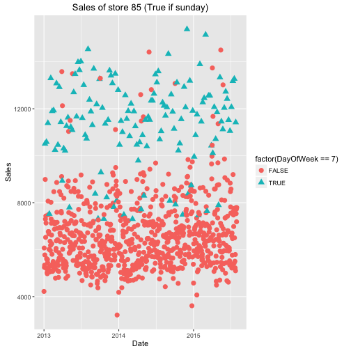
ggplot(train[Store == 262],
       aes(x = Date, y = Sales,
           color = factor(DayOfWeek == 7), shape = factor(DayOfWeek == 7))) +
    geom_point(size = 3) + ggtitle("Sales of store 262 (True if sunday)")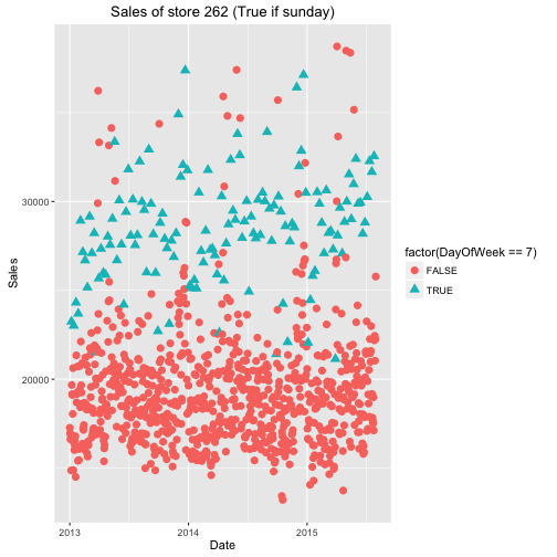
“That is not true in general. The variability of sales on sundays is quite high while the median is not:” Against my earlier intuition, the data says that high volume sales on Sundays are not typically common. They are unique to those stores with no 0 sales days.
ggplot(train[Sales != 0],
       aes(x = factor(DayOfWeek), y = Sales)) +
    geom_jitter(alpha = 0.1) +
    geom_boxplot(color = "yellow", outlier.colour = NA, fill = NA)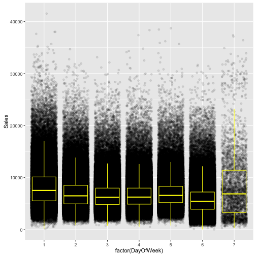
“The store file contains information about the stores that can be linked to
train and test via the store ID.”
Goal: observe the competition
as.yearmon() will convert a character string of “2002-8” to “Aug 2002” with class = “yearmon”. So when we paste together store\$CompetitionOpenSinceYear and store\$CompetitionOpenSinceMonth separated with a “-“ we end up with this original date format of %Y-%m which is converted to the proper format with as.yearmon(). Now we have the month and year that the competitor has been open since and we can take the difference between now and the year the store opened and plot this on a histogram. For example, if you enter, as.yearmon(“2016-6”) - as.yearmon(“2015-12”), R will output 0.5 (half a year).
The promos are slightly different because the time since is given in weeks along with the year. To change this to a proper date format we assume that the promo begins on the first day of the week and then format the dates like “2012-22-1” which is 31 weeks into the year 2012. The format can be read as “%Y-%U-%u”, which essentially says, year with century - week of the year as decimal number (00–53) - weekday as a decimal number (1–7, Monday is 1). A full list of all of these formatting types can be found at ?strptime. We then tell as.POSIXct() that this is the format of the date we will be feeding it, and it spits out dates like “2012-05-28 PDT”. Then we can look at a histogram of the differences between current time and those dates.
summary(store)## Store StoreType Assortment
## Min. : 1.0 Length:1115 Length:1115
## 1st Qu.: 279.5 Class :character Class :character
## Median : 558.0 Mode :character Mode :character
## Mean : 558.0
## 3rd Qu.: 836.5
## Max. :1115.0
##
## CompetitionDistance CompetitionOpenSinceMonth CompetitionOpenSinceYear
## Min. : 20.0 Min. : 1.000 Min. :1900
## 1st Qu.: 717.5 1st Qu.: 4.000 1st Qu.:2006
## Median : 2325.0 Median : 8.000 Median :2010
## Mean : 5404.9 Mean : 7.225 Mean :2009
## 3rd Qu.: 6882.5 3rd Qu.:10.000 3rd Qu.:2013
## Max. :75860.0 Max. :12.000 Max. :2015
## NA's :3 NA's :354 NA's :354
## Promo2 Promo2SinceWeek Promo2SinceYear PromoInterval
## Min. :0.0000 Min. : 1.0 Min. :2009 Length:1115
## 1st Qu.:0.0000 1st Qu.:13.0 1st Qu.:2011 Class :character
## Median :1.0000 Median :22.0 Median :2012 Mode :character
## Mean :0.5121 Mean :23.6 Mean :2012
## 3rd Qu.:1.0000 3rd Qu.:37.0 3rd Qu.:2013
## Max. :1.0000 Max. :50.0 Max. :2015
## NA's :544 NA's :544table(store$StoreType)##
## a b c d
## 602 17 148 348table(store$Assortment)##
## a b c
## 593 9 513# There is a connection between store type and type of assortment
table(data.frame(Assortment = store$Assortment, StoreType = store$StoreType))## StoreType
## Assortment a b c d
## a 381 7 77 128
## b 0 9 0 0
## c 221 1 71 220hist(store$CompetitionDistance, 100)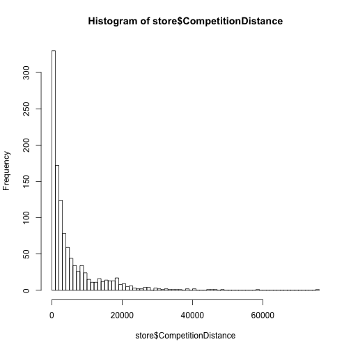
# Convert the CompetitionOpenSince... variables to one Date variable
store$CompetitionOpenSince <- as.yearmon(paste(store$CompetitionOpenSinceYear,
                                               store$CompetitionOpenSinceMonth, sep = "-"))
# One competitor opened 1900
hist(as.yearmon("2016-6") - store$CompetitionOpenSince, 100,
     main = "Years since opening of nearest competition")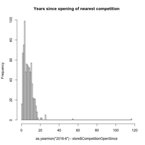
# Convert the Promo2Since... variables to one Date variable
# Assume that the promo starts on the first day of the week
store$Promo2Since <- as.POSIXct(paste(store$Promo2SinceYear,
                                   store$Promo2SinceWeek, 1, sep = "-"),
                             format = "%Y-%U-%u")
hist(as.numeric(as.POSIXct("2016-06-01", format = "%Y-%m-%d") - store$Promo2Since),
     100, main = "Days since start of promo2")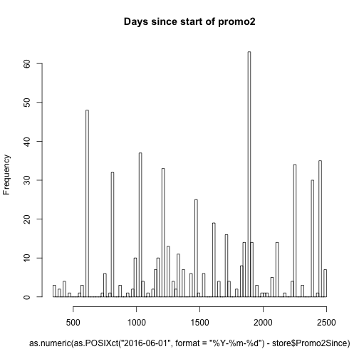
table(store$PromoInterval)##
## Feb,May,Aug,Nov Jan,Apr,Jul,Oct Mar,Jun,Sept,Dec
## 544 130 335 106“The stores with promos tend to make lower sales. This does not necessary mean that the promos don’t help or are counterproductive. They are possibly measures that are taken mainly by stores with low sales in the first place:”
merge() does pretty much the same thing something like left_join() would do from the dplyr package. This is typically where I tend towards when I’m joining dataframes, but here merge() is used.
# Merge store and train
train_store <- merge(train, store, by = "Store")
ggplot(train_store[Sales != 0], aes(x = factor(PromoInterval), y = Sales)) +
    geom_jitter(alpha = 0.1) +
    geom_boxplot(color = "yellow", outlier.colour = NA, fill = NA)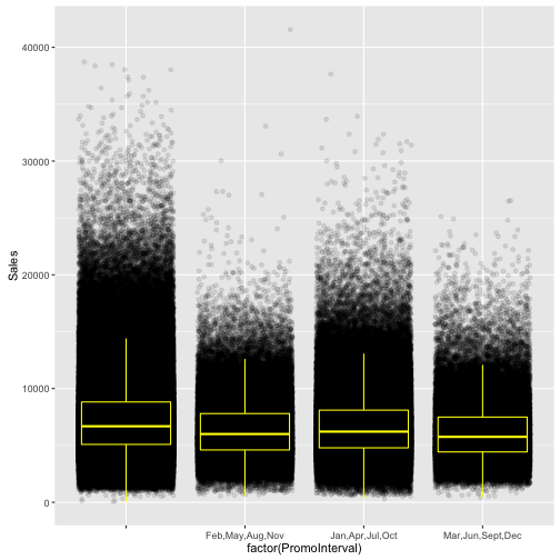
“The different store types and assortment types imply different overall levels of sales and seem to be exhibiting different trends:”
ggplot(train_store[Sales != 0],
       aes(x = as.Date(Date), y = Sales, color = factor(StoreType))) +
    geom_smooth(size = 2)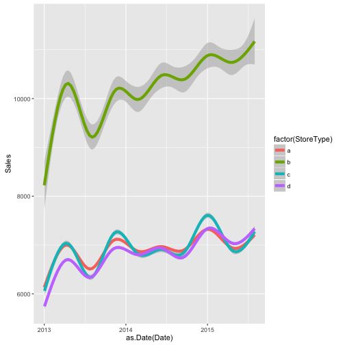
ggplot(train_store[Customers != 0],
       aes(x = as.Date(Date), y = Customers, color = factor(StoreType))) +
    geom_smooth(size = 2)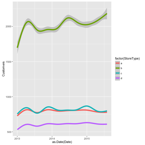
ggplot(train_store[Sales != 0],
       aes(x = as.Date(Date), y = Sales, color = factor(Assortment))) +
    geom_smooth(size = 2)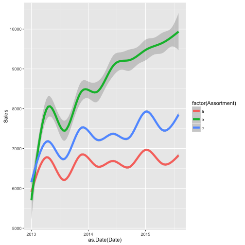
ggplot(train_store[Sales != 0],
       aes(x = as.Date(Date), y = Customers, color = factor(Assortment))) +
    geom_smooth(size = 2)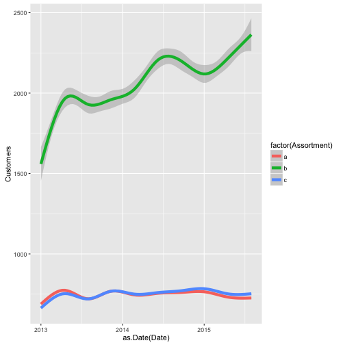
“The effect of the distance to the next competitor is a little counterintuitive. Lower distance to the next competitor implies (slightly, possibly not significantly) higher sales. This may occur (my assumption) because stores with a low distance to the next competitor are located in inner cities or crowded regions with higher sales in general. Maybe the effects of being in a good / bad region and having a competitor / not having a competitor cancel out:”
We used aggregate() earlier to calculate means across individual stores. Recall that it splits up the data into subsets and applies some summary statistic for each group. In this case, we take the elements of train_store where sales are not 0 and there is no NA value in the CompetitionDistance column, then we take only the Sales column within that subset of the data. We will calculate the mean of the sales across these data, but grouped by the competition distance, which if you look at the data are static groups of distances (i.e. 310, 1070, 960, etc.).
We then assign new column names to our dataframe by c() concatenating two character strings as shown below and assigning it to colnames(salesByDist).
Then we look at the log(CompetitionDistance) and log(MeanSales). We take the logs of each because without doing that the data is quite skewed. We have most of our data between 0 and 40000 and then a few outliers which alters the viewing of the graph. Taking the logs fixes this immediately.
salesByDist <- aggregate(train_store[Sales != 0 & !is.na(CompetitionDistance)]$Sales,
               by = list(train_store[Sales != 0 & !is.na(CompetitionDistance)]$CompetitionDistance), mean)
colnames(salesByDist) <- c("CompetitionDistance", "MeanSales")
ggplot(salesByDist, aes(x = log(CompetitionDistance), y = log(MeanSales))) +
    geom_point() + geom_smooth()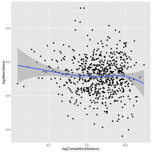
“A missing value for CompetitionDistance doesn’t necessarily mean that there is
no competiton. Maybe that data was just not collected, yet. There is no obvious
connection between sales and having NA as CompetitionDistance:”
A factor variable is created here, factor(!is.na(CompetitionOpenSinceYear)), of whether or not there is a listed competitor. !is.na() means that if there is not an NA, it will read TRUE.
ggplot(train_store[Sales != 0],
       aes(x = factor(!is.na(CompetitionOpenSinceYear)), y = Sales)) +
    geom_jitter(alpha = 0.1) +
    geom_boxplot(color = "yellow", outlier.colour = NA, fill = NA) +
    ggtitle("Any competition?")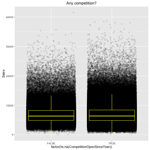
Goal: what happens when a competitor opens nearby?
“So what happens if a competitor opens? In order to assess this effect we fetch
data from all stores that first have NA as CompetitorDistance and later some
value. Only the month, not the date, of the opening of the competitor is known
so we need a rather large window to see the effect (100 days). 147 stores
had a competitor move into their area during the available time span. The
competition leaves a ‘dent’ in the sales which looks a little different
depending on the chosen timespan so I wouldn’t like to argue about statistical
significance based on this plot alone. It’s informative to look at anyway:”
First, we order all of the data by date.
Then we write a function that takes store numbers and outputs only those stores that had a change in competition and then look at 100 days before and after the competition comes in. So function(s) shows that we are about to define a function. We then assign an object, x, with the data values of one individual store specified by the function argument. Remember, this function takes a store number as its argument. We want to know if the competition’s open date is longer than that of the store itself. So daysWithComp is True if the competition date is after the date the store opened. Then we want to know if we got any True values for the logical statement, x\$CompetitionOpenSince >= x\$DateYearmon, according to that specific store. If there are False values, if (any(!daysWithComp)), then we want to find where the TRUEs meet the FALSEs, or in other words where head(which(!daysWithComp), 1) - 1 is not equal to 0. We also want 100 days before the store opens so we only want those where there are at least 100 TRUEs before we hit FALSEs, if (compOpening > timespan…), and also where there are at least 100 FALSEs, (…& compOpening < (nrow(x) - timespan)). Then we take 100 elements before and after the switch between TRUE to FALSE and only those elements of x, x[(compOpening - timespan):(compOpening + timespan), ], then we return the entire store data for the ones that fit our criteria.
# Sales before and after competition opens
train_store$DateYearmon <- as.yearmon(train_store$Date)
train_store <- train_store[order(Date)]
timespan <- 100 # Days to collect before and after Opening of competition
beforeAndAfterComp <- function(s) {
    x <- train_store[Store == s]
    daysWithComp <- x$CompetitionOpenSince >= x$DateYearmon
    if (any(!daysWithComp)) {
        compOpening <- head(which(!daysWithComp), 1) - 1
        if (compOpening > timespan & compOpening < (nrow(x) - timespan)) {
           x <- x[(compOpening - timespan):(compOpening + timespan), ]
            x$Day <- 1:nrow(x)
            return(x)
        }
    }
}
Now we can just grab those stores where there are no NA values !is.na() and then just take one store number from each using unique() and apply our function on each store. Now do.call(rbind, temp) just runs through this whole list and ignores the NULL values and rowbinds the data that exists. The length of the unique store values turns out to be 147 so those are the stores that had no competition when they opened but then had competition open at least 100 days after opening and 100 days before current. Then we see this graphic below.
temp <- lapply(unique(train_store[!is.na(CompetitionOpenSince)]$Store), beforeAndAfterComp)
temp <- do.call(rbind, temp)
# 147 stores first had no competition but at least 100 days before the end
# of the data set
length(unique(temp$Store))
## [1] 147ggplot(temp[Sales != 0], aes(x = Day, y = Sales)) +
geom_smooth() +
ggtitle(paste("Competition opening around day", timespan))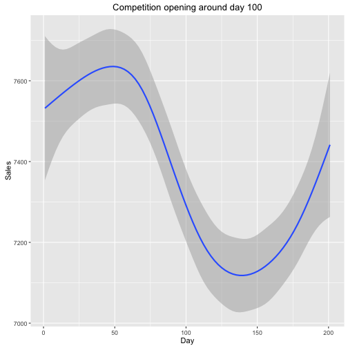
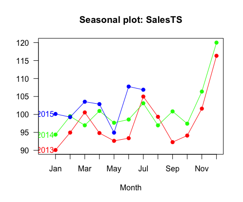
Goal: observe seasonality of sales
“The seasonplot is adapted from spsrini (edit: Replace sum and show sales in relation to mean daily sales of a store which better accounts for missing data / closed stores):”
First we break up the date comlumn into year and month. Then we assign StoreMean to be the mean of Sales organized by Store number. temp is now given this new variable MonthlySalesMean which is defined on the fly and then listed beside year and month. Typically we can only list one variable in the by = argument, but using the ‘.’ dot before the parentheses tells R to recognize the names of the variables and not their current value, allowing for more than one variable to be called together. The code still runs properly without the initial ‘.’ before MonthlySalesMean, but the variable name is not recognized.
temp <- train
temp$year <- format(temp$Date, "%Y")
temp$month <- format(temp$Date, "%m")
temp[, StoreMean := mean(Sales), by = Store]
temp <- temp[, .(MonthlySalesMean = mean(Sales / (StoreMean)) * 100),
             by = .(year, month)]
temp <- as.data.frame(temp)
ts() creates a time series object based on a starting point and the frequency of observations per unit of time. This is applied to the temp\$MonthlySalesMean data, and then to create a plot we use three different colors from the rainbow color set because we have three years, 2013, 2014, 2015. Then seasonplot(), which is kind of a relatively obscure function within the forecast package, is used to complete the graph.
SalesTS <- ts(temp$MonthlySalesMean, start=2013, frequency=12)
col = rainbow(3)
seasonplot(SalesTS, col=col, year.labels.left = TRUE, pch=19, las=1)